K-Means Clustering Algorithm
In this page, we will learn What is K-Means Algorithm?, How does the K-Means Algorithm Work?, How to choose the value of K number of clusters in K-means Clustering?, Elbow Method, Python Implementation of K-means Clustering Algorithm, Finding the optimal number of clusters using the elbow method.
K-Means Clustering is an unsupervised learning approach used in machine learning and data science to solve clustering problems. We will study what the K-means clustering method is, how it works, and how to implement it in Python in this topic.
What is K-Means Algorithm?
Unsupervised Learning algorithm K-Means Clustering divides the unlabeled dataset into various clusters. K specifies the number of pre-defined clusters that must be produced during the process; for example, if K=2, two clusters will be created, and if K=3, three clusters will be created, and so on.
“It is an iterative algorithm that divides the unlabeled dataset into k different clusters in such a way that each dataset belongs only one group that has similar properties.”
It allows us to cluster data into different groups and provides a simple technique to determine the categories of groups in an unlabeled dataset without any training.
It's a centroid-based algorithm, which means that each cluster has its own centroid. The main goal of this technique is to reduce the sum of distances between data points and the clusters that they belong to.
The technique takes an unlabeled dataset as input, separates it into a k-number of clusters, and continues the procedure until no better clusters are found. In this algorithm, the value of k should be predetermined.
The k-means clustering algorithm primarily accomplishes two goals:
- Iteratively determines the optimal value for K center points or centroids.
- Each data point is assigned to the k-center that is closest to it. A cluster is formed by data points that are close to a specific k-center.
As a result, each cluster contains datapoints with certain commonality and is isolated from the others.
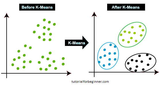
The K-means Clustering Algorithm is illustrated in the diagram below:
How does the K-Means Algorithm Work?
The following steps will describe how the K-Means algorithm works:
Step 1: To determine the number of clusters, choose the number K.
Step 2: Choose K locations or centroids at random. (It could be something different from the incoming dataset.)
Step 3: Assign each data point to the centroid that is closest to it, forming the preset K clusters.
Step 4: Reverse the third steps, reassigning each datapoint to the cluster's new nearest centroid.
Step 5: Determine the variance and reposition each cluster's centroid.
Step 6: If there is a reassignment, go to step-4; otherwise, move to FINISH.
Step 7: The model is now complete.
Consider the following graphic charts to better comprehend the preceding steps:
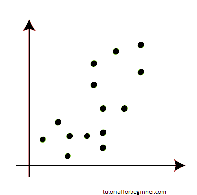
Suppose we have two variables M1 and M2. The x-y axis scatter plot of these two variables is given below:
- To identify the dataset and place it into various clusters, we'll use the number k of clusters, i.e., K=2. That is, we will attempt to divide these datasets into two distinct clusters.
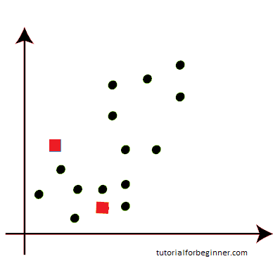
- To build the cluster, we must choose some random k points or centroid. These points can be from the dataset or they can come from anywhere else. As a result, we've chosen the two points below as k points, despite the fact that they're not in our dataset. Consider the following illustration:
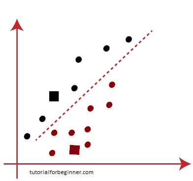
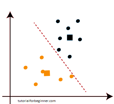
- Now we'll assign each scatter plot data point to the nearest K-point or centroid. We'll figure it out using the arithmetic we've learned about calculating distances between two spots. As a result, we'll draw a line connecting both centroids. Consider the following illustration:
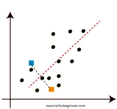
The points on the left side of the line are close to the K1 or blue centroid, and the points on the right side of the line are close to the yellow centroid, as shown in the above image. To make them easier to see, we'll color them blue and yellow.
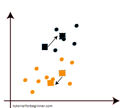
We'll repeat the process by selecting a new centroid because we need to discover the closest cluster. We will compute the center of gravity of these centroids in order to find new centroids, and we will do it as follows:
- Then, for each datapoint, we'll reassign it to the new centroid. We'll go through the same steps as before to identify a median line. The median will look like this:
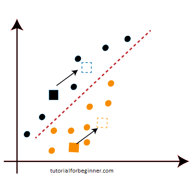
- Then, for each datapoint, we'll reassign it to the new centroid. We'll go through the same steps as before to identify a median line. The median will look like this:
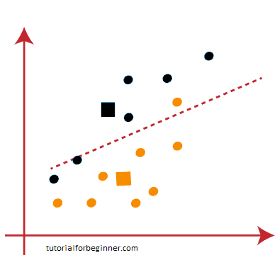
One yellow point is on the left side of the line, and two blue points are on the right side of the line, as seen in the above image. As a result, new centroids will be allocated to these three sites.
As reassignment has occurred, we will proceed to step 4, which is the search for new centroids or K-points.
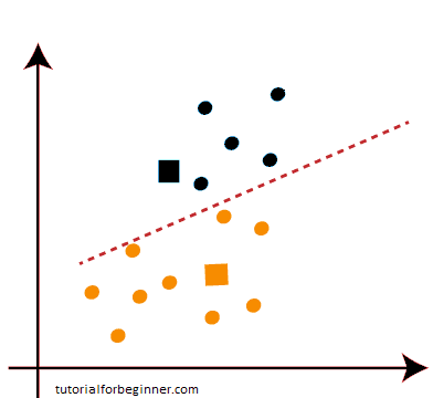
- We'll repeat the process by determining the center of gravity of centroids, resulting in new centroids that look like the ones below:
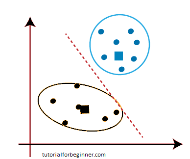
- We'll redraw the median line and reassign the data points now that we have the new centroids. As a result, the image will be:
- As we can see in the graphic above, there are no data points on either side of the line that are dissimilar, indicating that our model is established. Consider the following illustration:
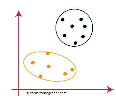
Because our model is complete, we can now delete the assumed centroids, resulting in the two final clusters shown below:
How to choose the value of "K number of clusters" in K-means Clustering?
The K-means clustering algorithm's performance is dependent on the very efficient clusters it creates. However, determining the ideal number of clusters is a difficult process. There are several methods for determining the best number of clusters, but we will focus on the most appropriate approach for determining the number of clusters or K value. The procedure is as follows:
Elbow Method
One of the most prominent methods for determining the ideal number of clusters is the Elbow approach. This approach makes use of the WCSS value notion. Within Cluster Sum of Squares (WCSS) is a term that describes the total variations within a cluster. The formula for calculating the WCSS value (for three clusters) is as follows:
WCSS= ∑Pi in Cluster1 distance(PiC1)2 + ∑Pi in Cluster2 distance(PiC2)2+ ∑Pi in CLuster3 distance(PiC3)2
In the above formula of WCSS,
∑Pi in Cluster1 distance(PiC1) 2 : It is the sum of the square of the distances between each data point and its centroid within a cluster1 and the same for the other two terms.
We can use any method, such as the Euclidean or Manhattan distance, to calculate the distance between data points and the centroid.
The elbow method uses the methods below to determine the ideal cluster value:
- On a given dataset, it performs K-means clustering for various K values (ranges from 1-10).
- Calculates the WCSS score for each value of K.
- Plots a line between estimated WCSS values and K clusters.
- If a sharp point of bend or a plot point resembles an arm, that point is the optimal K value
Because the graph depicts a sharp bend that resembles an elbow, it is referred to as the elbow method. The elbow method's graph looks somewhat like this:
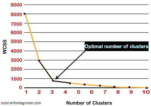
[ Note: the number of clusters equal to the number of data points can be chosen. If we choose a number of clusters equal to the number of data points, the WCSS value becomes zero, and the plot ends there. ]
Python Implementation of K-means Clustering Algorithm
We reviewed the K-means method in the previous part; now let's look at how it may be implemented in Python.
Before we get started, let's figure out what kind of difficulty we're dealing with. So, we have a Mall Customers dataset, which contains information about customers who visit the mall and spend money there.
Customer Id, Gender, Age, Annual Income ($), and Spending Score are all included in the dataset (which is the calculated value of how much a customer has spent in the mall, the more the value, the more he has spent). We need to calculate some patterns from this dataset because it is an unsupervised method and we don't know exactly what to calculate.
The steps to be followed for the implementation are given below:
- Data Pre-processing
- Finding the optimal number of clusters using the elbow method
- Training the K-means algorithm on the training dataset
- Visualizing the clusters
Step-1: Data pre-processing Step
The initial phase, as with our previous topics of regression and classification, will be data pre-processing. However, it will be distinct from existing models for the clustering problem. Let's talk about it:
- Importing Libraries: First, we'll import the libraries for our model, which is part of data pre-processing, as we did in previous topics. The code is as follows:
   #importing libraries
   import numpy as nm
   import matplotlib.pyplot as mtp
   import pandas as pd
Numpy is used to do mathematical calculations, matplotlib is used to plot the graph, and pandas is used to manage the dataset in the code above.
- Importing the Dataset: After that, we'll import the dataset we'll be working with. We're going to use the Mall_Customer_data.csv dataset for this. The following code can be used to import it:
   #Importing the dataset
   dataset = pd.read_csv('Mall_Customers_data.csv')
By executing the above lines of code, we will get our dataset in the Spyder IDE. The dataset looks like the below image:
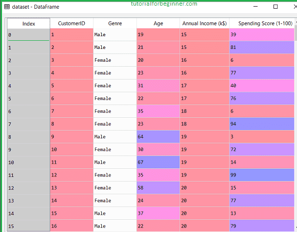
We need to detect some trends in the dataset mentioned above.
- Extracting Independent Variables
Because this is a clustering problem and we have no notion what to determine, we don't require any dependent variables for the data pre-processing stage. So, for the matrix of features, we'll merely add a line of code.
x = dataset.iloc[:, [3, 4]].values
As can be seen, we are just extracting the third and fourth features. It's because we need a 2d plot to visualize the model, and some features, such as customer id, aren't required.
Step-2: Finding the optimal number of clusters using the elbow method
In the second phase, we'll try to figure out how many clusters are best for our clustering problem. As previously stated, we will employ the elbow method in this instance.
The elbow method, as we all know, draws the plot by plotting WCSS values on the Y-axis and the number of clusters on the X-axis using the WCSS idea. As a result, we'll calculate the WCSS value for various k values ranging from 1 to 10. The code for it is as follows:
   #finding optimal number of clusters using the elbow method
   from sklearn.cluster import KMeans
   wcss_list = []  #Initializing the list for the values of WCSS

   #Using for loop for iterations from 1 to 10.
   for i in range(1, 11):
    kmeans = KMeans(n_clusters=i, init='k-means++', random_state = 42)
    kmeans.fit(x)
    wcss_list.append(kmeans.inertia_)
   mtp.plot(range(1, 11), wcss_list)
   mtp.title('The Elobw Method Graph')
   mtp.xlabel('Number of clusters(k)')
   mtp.ylabel('wcss_list')
   mtp.show()
To build the clusters, we used the KMeans class of the sklearn. cluster package, as seen in the preceding code.
Next, we established the wcss list variable to construct an empty list that will hold the wcss value computed for various values of k ranging from 1 to 10.
Following that, we initialized the for loop for iteration on a distinct value of k ranging from 1 to 10; because for loops in Python do not include the outbound limit, we used 11 to include the 10th number.
The rest of the code is identical to what we did in previous subjects, in that we fitted the model to a matrix of features and then plotted the graph between cluster number and WCSS.
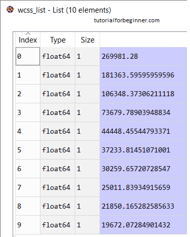
Output: After executing the above code, we will get the below output:
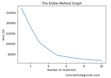
From the above plot, we can see the elbow point is at 5. So the number of clusters here will be 5.
Step- 3: Training the K-means algorithm on the training dataset
We can now train the model on the dataset because we know how many clusters there are. We'll use the same two lines of code to train the model as we did in the previous section, but instead of using I we'll use 5, because there are five clusters to construct. The code is as follows:
  #training the K-means model on a dataset
  kmeans = KMeans(n_clusters = 5, init = 'k-means++', random_state = 42)
  y_predict= kmeans.fit_predict(x)
The first line is the same as before for generating a KMeans class object.
To train the model, we created the dependent variable y predict in the second line of code.
The y predict variable is obtained by running the above lines of code. In the Spyder IDE, we can inspect it using the variable explorer option. We can now compare the y predict values to the values in our original dataset. Consider the below image:
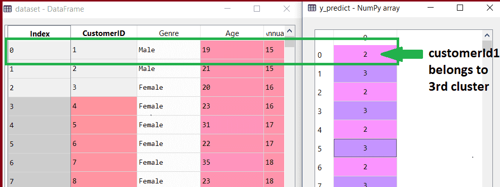
From the above image, we can now relate that the CustomerID 1 belongs to a cluster
3(as index starts from 0, hence 2 will be considered as 3), and 2 belongs to cluster 4, and so on.
Step-4: Visualizing the Clusters
The clusters must then be seen as the final stage. Because our model has five clusters, we'll look at each one separately.
To visualize the clusters will use scatter plot using mtp.scatter() function of matplotlib.
   #visulaizing the clusters
   mtp.scatter(x[y_predict == 0, 0], x[y_predict == 0, 1], s = 100, c = 'blue', label = 'Cluster 1') #for first cluster
   mtp.scatter(x[y_predict == 1, 0], x[y_predict == 1, 1], s = 100, c = 'green', label = 'Cluster 2') #for second cluster
   mtp.scatter(x[y_predict== 2, 0], x[y_predict == 2, 1], s = 100, c = 'red', label = 'Cluster 3') #for third cluster
   mtp.scatter(x[y_predict == 3, 0], x[y_predict == 3, 1], s = 100, c = 'cyan', label = 'Cluster 4') #for fourth cluster
   mtp.scatter(x[y_predict == 4, 0], x[y_predict == 4, 1], s = 100, c = 'magenta', label = 'Cluster 5') #for fifth cluster
   mtp.scatter(kmeans.cluster_centers_[:, 0], kmeans.cluster_centers_[:, 1], s = 300, c = 'yellow', label = 'Centroid')
   mtp.title('Clusters of customers')
   mtp.xlabel('Annual Income (k$)')
   mtp.ylabel('Spending Score (1-100)')
   mtp.legend()
   mtp.show()
We have written code for each cluster, spanning from 1 to 5, in the lines above. The mtp.scatter's initial coordinate, x[y_predict == 0, 0], contains the x value for displaying the matrix of feature values, with the y_predict range from 0 to 1.
Output:
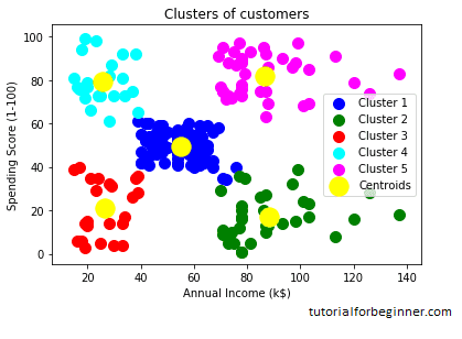
The generated graphic clearly displays the five distinct clusters in various hues. The clusters are built by two dataset parameters: customer annual income and spending. Colors and labels can be changed to suit your needs or preferences. Some points can be gleaned from the above patterns, which are listed below:
- Cluster1 depicts consumers with an average salary and average spending, allowing us to classify them as cautious.
- Cluster2 depicts customers with a high income but low spending, allowing us to classify them as cautious.
- Cluster3 demonstrates low income as well as low spending, indicating that they are prudent.
- Cluster4 depicts customers with low income but high spending, indicating that they are careless.
- Cluster5 identifies customers with high wealth and high spending, allowing them to be classified as target customers, who can be the most profitable for the mall owner.