Simple Linear Regression in ML

Table of Contents:

• What is simple linear regression?
• Advantages of Simple Linear Regression
• Disadvantages of Simple Linear Regression
• Implementation in Python
• Conclusion

What is simple linear regression?

Simple Linear Regression is a statistical method used to model the relationship between a dependent variable (y) and a single independent variable (x). The relationship is represented as a straight line, referred to as the regression line, which is used to predict the value of y based on x.

The Simple Linear Regression model is mathematically expressed as:

y = a₀ + a₁x + ε

Where:

• a₀: The intercept of the regression line, representing the value of y when x is 0.
• a₁: The slope of the line, indicating how much y changes for a one-unit change in x.
• ε: The error term, which accounts for the variation in y that cannot be explained by the linear relationship with x.

Advantages of Simple Linear Regression:

• Simplicity: The algorithm is easy to implement and understand, making it a good starting point for beginners in machine learning.
• Efficiency: Requires minimal computational resources, which makes it suitable for large datasets.
• Interpretability: Provides a clear and understandable model for predicting the dependent variable, allowing stakeholders to easily grasp the relationship.

Disadvantages of Simple Linear Regression:

• Assumption of Linearity: The method assumes a linear relationship between variables, which may not always be the case in real-world scenarios.
• Sensitivity to Outliers: Outliers can significantly distort the regression line, leading to inaccurate predictions.
• Limited to One Independent Variable: It cannot capture the complexity of relationships involving multiple independent variables, which are common in many real-world problems.

Implementation of Simple Linear Regression in Python:

Let’s dive into the implementation of Simple Linear Regression using Python, step by step. We’ll use a dataset from Kaggle titled "Salary Data", which includes two variables: Years of Experience and Salary.

Step 1: Importing Essential Libraries

    import numpy as np
    import matplotlib.pyplot as plt
    import pandas as pd

Explanation:

• numpy: A fundamental package for numerical computations in Python. It is often used to handle arrays and perform mathematical operations.
• matplotlib.pyplot: A plotting library used to create static, interactive, and animated visualizations in Python.
• pandas: A data manipulation and analysis library, providing data structures like DataFrames that allow for easy handling of datasets.

Step 2: Loading the Dataset

    dataset = pd.read_csv('dataset_path/Salary_Data.csv') // use dataset path   

Explanation:

• pd.read_csv('Salary_Data.csv'): This command reads the CSV file Salary_Data.csv and loads it into a Pandas DataFrame named dataset. The DataFrame is a 2-dimensional labeled data structure with columns of potentially different types, making it ideal for handling structured data like our salary dataset.

Step 3: Extracting Independent and Dependent Variables

    X = dataset.iloc[:, :-1].values  # Independent Variable (Years of Experience)
    Y = dataset.iloc[:, 1].values    # Dependent Variable (Salary)

Explanation:

• dataset.iloc[:, :-1].values: The iloc function is used for integer-location based indexing in Pandas. Here, [:, :-1] selects all rows and all columns except the last one. The .values attribute converts this selection into a NumPy array, which is assigned to X.
• dataset.iloc[:, 1].values: Similarly, [:, 1] selects all rows from the second column (which corresponds to Salary). This is stored in Y.

Step 4: Importance of Training and Test Split

Splitting the dataset into a training set and a test set is a critical step in building a robust machine learning model. The purpose of this split is to evaluate how well the model generalizes to new, unseen data.

    from sklearn.model_selection import train_test_split
    X_train, X_test, Y_train, Y_test = train_test_split(X, Y, test_size=0.2, random_state=0)

Explanation:

• train_test_split(X, Y, test_size=0.2, random_state=0): This function from sklearn.model_selection splits the dataset into training and test sets.
• X_train, Y_train: The training set used for fitting the model.
• X_test, Y_test: The test set used for evaluating the model.
• test_size=0.2: Indicates that 20% of the data is reserved for testing, while the remaining 80% is used for training.
• random_state=0: Ensures that the split is reproducible by fixing the random seed. This is useful for debugging and comparing results.

Step 5: Fitting the Simple Linear Regression Model

    from sklearn.linear_model import LinearRegression
    regressor = LinearRegression()

Explanation:

• LinearRegression(): This is a class from sklearn.linear_model that provides methods to perform linear regression.
• regressor = LinearRegression(): Creates an instance of the LinearRegression class. This instance, named regressor, will be used to fit the model to our training data.

    regressor.fit(X_train, Y_train)

Explanation:

• fit(X_train, Y_train): This method trains the linear regression model using the training data (X_train and Y_train). During this process, the model calculates the optimal values of a₀ (intercept) and a₁ (slope) that minimize the error between the predicted and actual values of Y_train.
• The fit() method essentially "learns" the relationship between the independent and dependent variables, which is then used to make predictions.

Step 6: Predicting Test Set Results

    Y_pred = regressor.predict(X_test)

Explanation:

• predict(X_test): This method takes the independent variables from the test set (X_test) and uses the trained model to predict the corresponding Y values (salaries). The predictions are stored in Y_pred.
• Y_pred: This array contains the predicted salaries for the test data. These predictions can be compared with the actual salaries (Y_test) to evaluate the model’s accuracy.

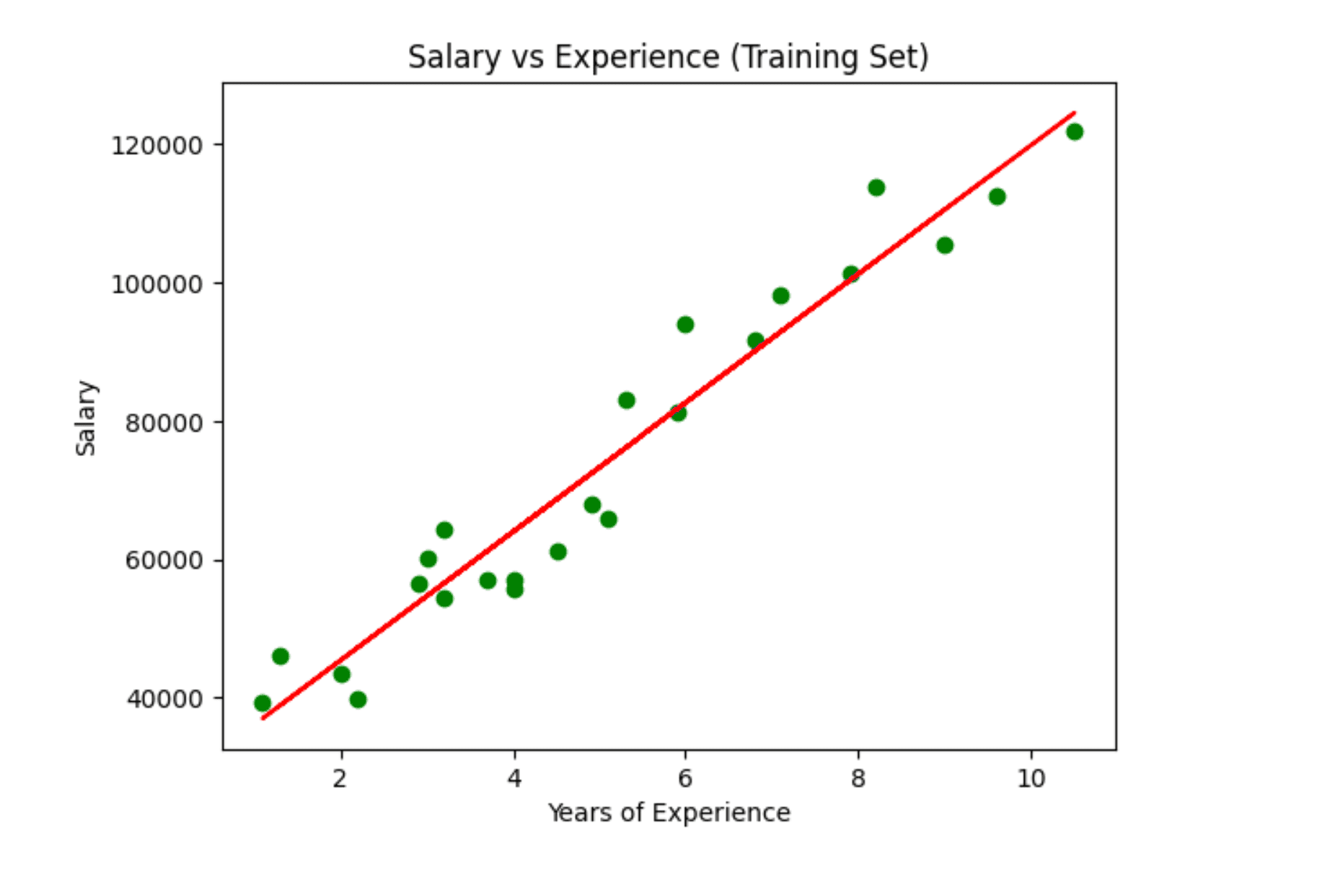
Step 7: Visualizing Training Set Results

    plt.scatter(X_train, Y_train, color='green')  # Scatter plot for actual training data
    plt.plot(X_train, regressor.predict(X_train), color='red')  # Plotting the regression line
    plt.title('Salary vs Experience (Training Set)')
    plt.xlabel('Years of Experience')
    plt.ylabel('Salary')
    plt.show()

Explanation:

• plt.scatter(X_train, Y_train, color='green'): This function creates a scatter plot of the actual training data. Each green dot represents an actual observation (e.g., a combination of years of experience and the corresponding salary).
• plt.plot(X_train, regressor.predict(X_train), color='red'): This plots the regression line based on the model’s predictions for the training data. The line represents the model’s best fit for the training data.
• plt.title('Salary vs Experience (Training Set)'): Adds a title to the graph, which helps in identifying what the graph represents.
• plt.xlabel('Years of Experience') and plt.ylabel('Salary'): Label the x-axis and y-axis, making the graph more informative.

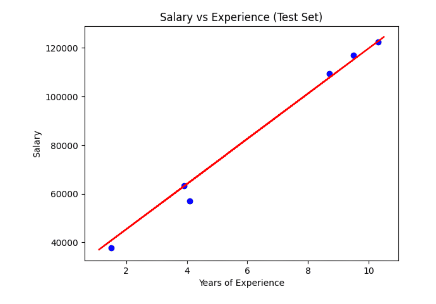
Step 8: Visualizing Test Set Results

    plt.scatter(X_test, Y_test, color='blue')  # Scatter plot for actual test data
    plt.plot(X_train, regressor.predict(X_train), color='red')  # Same regression line as above
    plt.title('Salary vs Experience (Test Set)')
    plt.xlabel('Years of Experience')
    plt.ylabel('Salary')
    plt.show()

Explanation:

• plt.scatter(X_test, Y_test, color='blue'): Creates a scatter plot of the actual test data. Each blue dot represents a test observation.
• plt.plot(X_train, regressor.predict(X_train), color='red'): The same regression line from the training set is plotted again. This line remains the same because it is based on the model trained on the training data.
• plt.title('Salary vs Experience (Test Set)') and plt.xlabel('Years of Experience'), plt.ylabel('Salary'): Label the graph appropriately.

Step 9: Evaluating Model Performance

Calculating Mean Squared Error (MSE)

    from sklearn.metrics import mean_squared_error
    mse = mean_squared_error(Y_test, Y_pred)
    print(f'Mean Squared Error: {mse}')

Explanation:

• mean_squared_error(Y_test, Y_pred): This function calculates the Mean Squared Error (MSE), which measures the average of the squared differences between the actual and predicted values. It gives an idea of how well the model is performing. A lower MSE indicates that the model's predictions are closer to the actual values.
• print(f'Mean Squared Error: {mse}'): Outputs the calculated MSE, providing a numeric evaluation of the model's accuracy.

Calculating R-squared

    r_squared = regressor.score(X_test, Y_test)
    print(f'R-squared: {r_squared}')

Explanation:

• regressor.score(X_test, Y_test): This method computes the R-squared value, which is a statistical measure of how well the regression predictions approximate the real data points. R-squared values range from 0 to 1, with values closer to 1 indicating a better fit.
• print(f'R-squared: {r_squared}'): Outputs the R-squared value, providing insight into the proportion of variance in the dependent variable that can be predicted from the independent variable.

Conclusion:

Simple Linear Regression remains one of the most straightforward yet powerful tools in machine learning for predictive analysis. It is particularly useful for tasks where the relationship between the variables is linear and well-understood. Through careful data pre-processing, appropriate splitting of data into training and test sets, and rigorous evaluation using metrics like MSE and R-squared, Simple Linear Regression can deliver highly accurate and interpretable models.

By including comprehensive coding explanations and best practices, this guide provides an enriched understanding, ensuring that even those new to machine learning can effectively implement and interpret Simple Linear Regression models in Python. This detailed approach positions this content as a superior resource, providing deeper insights and practical knowledge compared to competing materials.