Deep Learning Algorithms
In this Deep Learning Algorithms page, we will learn What is Deep Learning Algorithms?, Why Deep Learning is important?, Deep Learning Algorithms, Convolutional Neural Networks (CNNs), Long Short Term Memory Networks (LSTMs), Recurrent Neural Networks (RNNs), Generative Adversarial Networks (GANs), Radial Basis Function Networks (RBFNs), Multilayer Perceptrons (MLPs), Self Organizing Maps (SOMs), Deep Belief Networks (DBNs), Restricted Boltzmann Machines (RBMs), and summary.
What is Deep Learning Algorithm?
Deep learning is a type of machine learning and artificial intelligence that aims to intimidate individuals and their actions by mimicking specific aspects of how the human brain works to make wise decisions. It is a crucial component of data science to channel its modeling based on data-driven methods under statistical and predictive modeling. There must be some powerful forces that we often refer to as algorithms in order to drive such a human-like ability to adapt, learn, and perform accordingly.
Several layers of neural networks, which are nothing more than a collection of decision-making networks that are pre-trained to do a task, are dynamically constructed to run deep learning algorithms across them. Each of these is thereafter put through basic layered representations before moving on to the following layer. The majority of machine learning, however, is developed to perform quite well on datasets that have hundreds of features or columns. Machine learning frequently fails, whether a data set is organized or unstructured, primarily because it is unable to distinguish a 800x1000 RGB basic image. For a standard machine learning method to handle such depths, it becomes rather impractical. Deep learning comes into play here.
Why Deep Learning is important?
Deep learning algorithms are essential for identifying features and are capable of handling a sizable number of operations for both structured and unstructured data. However, because deep learning algorithms require access to enormous amounts of data in order to be effective, they may be overkill for some jobs that may involve difficult challenges. For instance, Imagenet, a well-liked deep learning image recognition program, has access to 14 million photos in its dataset-driven algorithms. It is a very thorough tool that established the highest standard for deep learning techniques that use photos as their dataset.
Deep learning algorithms are extremely progressive algorithms that gather knowledge about the image we previously discussed by processing it through each layer of the neural network. Due to the layers' strong sensitivity to low-level visual elements like edges and pixels, the merged layers use this information to create comprehensive representations by comparing it to earlier data. For instance, other deep-trained layers may be programmed to detect certain items like dogs, trees, kitchenware, etc., while the middle layer may be programmed to detect specific sections of the object in the shot.
Deep learning algorithms, however, are unable to generalize basic data if we spell out a simple task that includes less complexity and a data-driven resource. This is one of the key reasons why boosted tree models or linear models of deep learning are preferred. Simple models are designed to generate custom data quickly, detect fraudulent activity, and work with datasets that are less complicated and have fewer properties. Deep learning can be useful in a variety of situations, such as multiclass classification, even though it is typically not recommended. These situations require smaller, more organized datasets.
After that, let's look at some of the most significant deep learning algorithms that are provided below.
Deep Learning Algorithms
The Deep Learning Algorithms are as follows:
1. Convolutional Neural Networks (CNNs)
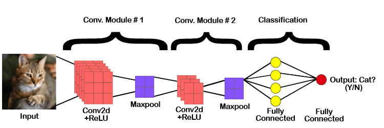
ConvNets, often referred to as CNNs, are primarily made up of numerous layers and are used mainly for object detection and image processing. It was first known as LeNet and was created by Yann LeCun in 1998. It was created back then to detect numerals and zip code characters. CNNs are widely used in anomaly detection, series forecasting, medical image processing, and satellite image identification.
In order to do convolutional operations, CNNs process the data by putting it through several layers and extracting features. Rectified Linear Units (ReLUs), which are part of the convolutional layer, are used to correct the feature map. These feature maps are corrected for the following feed using the pooling layer. Pooling is often a down-sampled sampling procedure that decreases the dimensionality of the feature map. Later, the output is produced as 2-D arrays made up of a single, long, continuous, and linear vector that has been flattened in the map. The following layer, known as the Fully Connected Layer, uses the flattened matrix or 2-D array that was obtained from the Pooling Layer as input to classify the image and identify it.
2. Long Short Term Memory Networks (LSTMs)
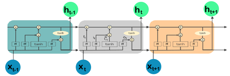
Recurrent neural networks (RNNs) with long-term dependent learning and adaptation capabilities are known as LSTMs. It can remember and recall information from the past for a longer time, and by default, this is its only behavior. Because LSTMs can hold onto memories or prior inputs, they are frequently utilized in time series predictions because they are built to retain information across time. This comparison is made due to their chain-like structure, which consists of four interconnected layers that communicate with one another in various ways. Along with time series prediction applications, they can be used to build voice recognizers, advance medicinal research, and create musical loops.
The LSTM operates through a series of events. First of all, they have a tendency to forget superfluous information acquired in the preceding condition. They then selectively update a subset of the cell-state values before generating a subset of the cell-state as an output. The diagram of how they work is below.
3. Recurrent Neural Networks (RNNs)
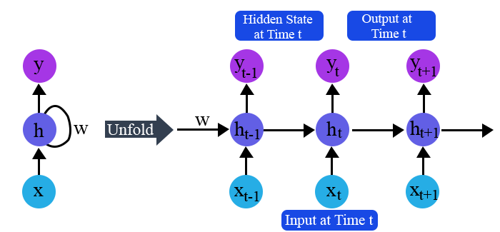
Recurrent neural networks, also known as RNNs, are made up of a cycle of directed connections that enables the current phase of RNNs to utilise the input from the LSTMs. Because these inputs are so deeply ingrained, the LSTMs' capacity for memorization allows them to be temporarily stored in the internal memory. As a result, RNNs rely on the inputs that LSTMs preserve and operate in accordance with the synchronization phenomena of LSTMs. RNNs are mostly used for data translation to machines, time series analysis, handwritten data recognition, and captioning of images.
When the time is defined as t, RNNs put output feeds at (t-1) time in accordance with the work strategy. At input time t+1, the output determined by t is then fed. Similar operations are carried out for all inputs, regardless of their length. RNNs have the additional property of storing historical data, so even if the model size is expanded, the input size remains constant. RNNs resemble this when they are fully unfolded.
4. Generative Adversarial Networks (GANs)
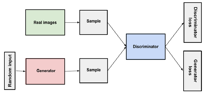
GANs are deep learning algorithms that produce new instances of data that closely resemble the training data. In a GAN, there are typically two parts: a generator that learns to produce fake data and a discriminator that adjusts by taking lessons from this fake data. Since they are widely employed to sharpen astronomical images and simulate gravitational dark matter, GANs have grown significantly in popularity over time. Additionally, by replicating 2D textures at a higher quality, such as 4K, video games can boost the visual appeal of their 2D textures. They are also employed in the production of lifelike cartoon characters, as well as the representation of human faces and 3D objects.
GANs simulate by creating and processing both fictitious and real data. The discriminator quickly learns to adapt and recognize this as false data throughout the training to grasp this data, while the generator produces various types of phony data. These results are then sent for updating by GANs. To picture how it works, think about the illustration below.
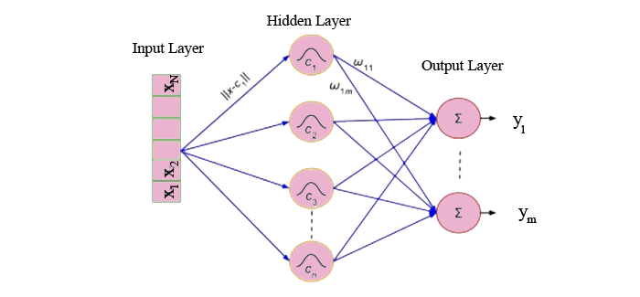
5. Radial Basis Function Networks (RBFNs)
Radial functions are used as activation functions in RBFNs, a subset of neural networks that employ a feed-forward methodology. Input, hidden, and output layers make up their three layers, which are mostly utilized for time-series prediction, regression analysis, and classification.
By analyzing the similarities found in the training data set, RBFNs do these tasks. Typically, they contain an input vector that sends these data into the input layer, validating the identification and disseminating results by comparing prior data sets.
The input layer's neurons are specifically sensitive to certain data, and the layer's nodes are effective at classifying the data class. Although they cooperate closely with the input layer, neurons are initially found in the hidden layer. The output's distance from the center of the neuron is inversely proportional to the Gaussian transfer functions in the hidden layer. The output layer consists of linear combinations of radial-based data where output is produced using Gaussian functions that are supplied as parameters to the neuron. Consider the illustration provided below to fully comprehend the procedure.
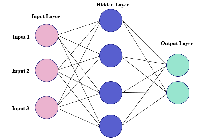
6. Multilayer Perceptrons (MLPs)
The foundation of deep learning technology is MLPs. It belongs to a group of feed-forward neural networks that have several perceptron-filled layers. These perceptrons each have a different activation function. Input and output layers in MLPs are also connected and have the same number of layers. Between these two strata, there is another layer that is still undiscovered. MLPs are primarily used to create voice and picture recognition software, as well as various kinds of translation software.
Data is fed into the input layer to begin the operation of MLPs. The layer's neurons come together to create a graph that creates a link that only goes in one direction. It is discovered that there is weight for this input data between the hidden layer and the input layer. Which nodes are ready to fire is determined by MLPs using activation functions. The tanh function, sigmoid, and ReLUs are some of these activation mechanisms. In order to produce the required output from the given input set, MLPs are mostly utilized to train the models and determine what kind of co-relation the layers are serving. To further understand, see the illustration below.
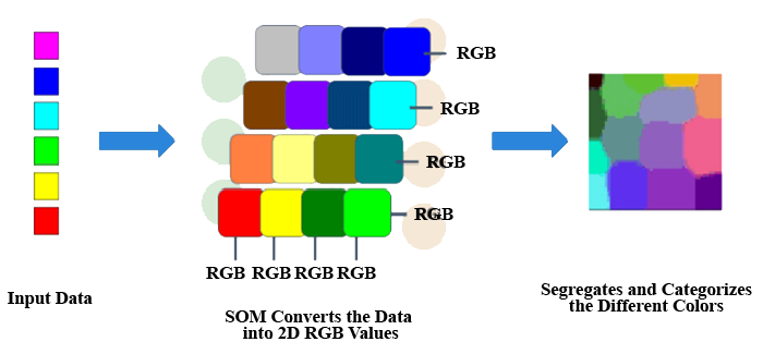
7. Self Organizing Maps (SOMs)
Teuvo Kohenen created SOMs in order to see data and comprehend its aspects using artificial, self-organizing neural networks. In order to solve problems, attempts are made to visualize data that is mostly impossible for people to see. Because this data is typically multidimensional, there are fewer opportunities for human error and involvement.
SOMs aid in data visualization by choosing random vectors from the provided training data after initializing the weights of various nodes. So that dependencies may be understood, they look at each node to determine the respective weights.
The best matching unit is used to choose the winning node (BMU). These winning nodes are later found by SOMs, but they gradually disappear from the sample vector. Therefore, there is a greater likelihood of identifying the weight and doing additional tasks the closer the node is to BMU. To make sure that no node closer to BMU is overlooked, numerous iterations are also performed. The RGB color combinations that we employ in our daily chores are one example of such. To comprehend how they work, consider the illustration below.
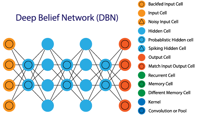
8. Deep Belief Networks (DBNs)
Because DBNs comprise multiple layers of latent and stochastic variables, they are also known as generative models. Because the latent variable has binary values, it is referred to as a hidden unit. Because the RGM layers are piled on top of one another to establish communication between earlier and later layers, DBNs are also known as Boltzmann Machines. Applications like video and image identification as well as the capture of moving objects use DBNs.
Algorithms that are greedy power DBNs. The most common method by which DBNs operate is by leaning through a top-down strategy to create weights in layers. On the top hidden two-layer, DBNs employ a step-by-step Gibbs sampling method. Then, using a model that adheres to the ancestral sampling approach, these steps take a sample from the discernible units. Following the bottom-up pass strategy, DBNs learn from the values that are contained in the latent value of each layer.
9. Restricted Boltzmann Machines (RBMs)
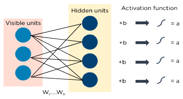
RBMs are stochastic neural networks that learn from the probability distribution in the supplied input set. They were created by Geoffrey Hinton. This algorithm is mostly employed in the areas of topic modeling, regression, and classification, as well as in the reduction of dimension. The visible layer and the hidden layer are the two layers that make up RBIs. Both of these layers have bias units attached to nodes that produce the output and are connected via hidden units. RBMs typically consist of two phases: a forward pass and a backward pass.
By taking inputs and converting them to numbers, RBMs carry out their duty of encoding inputs in the forward pass. Every input is weighted by RBMs, and the backward pass takes these weights and further transforms them into reconstructed inputs. Both of these translated inputs are afterwards mixed with their respective weights. These inputs are subsequently sent to the visible layer, where activation takes place and an output that is simple to reconstruct is produced. Consider the graphic below to get a better idea of this procedure.
Auto-encoders
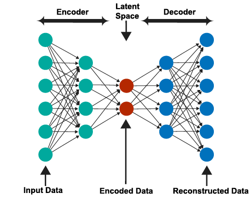
A unique kind of neural network called an auto-encoder finds inputs and outputs that are typically identical. It was created largely to address issues with unsupervised learning. Highly trained neural networks called auto-encoders reproduce the data. Because of that, the input and output are typically the same. They are employed to do various tasks, including population prediction, image processing, and drug discovery.
The encoder, the code, and the decoder are the three parts that make up an auto-encoder. The design of auto-encoders allows them to take in inputs and convert them into a variety of representations. Reconstructing the original input is a more accurate method of copying it. They accomplish this by reducing the size and encoding the image or input. If the image is not clearly visible, it is sent to the neural network for explanation. The image that has been made clearer is then referred to as a reconstruction image, and it is equally accurate as the original image. See the illustration provided below to comprehend this intricate process.
Summary
In this article, deep learning and the algorithms that support it are mostly used. In the beginning, we discovered how deep learning uses vision to alter the world at a rapid pace in order to develop intelligent software that can replicate it and act similarly to the human brain. In a later section of this essay, we will learn about some of the most popular deep learning algorithms and the elements that power them. Typically, a person must have a strong understanding of the mathematical functions presented in some of the algorithms in order to comprehend these algorithms. These functions are so important that the calculations made using these functions and formulas are what these algorithms rely on the most to function. All of these methods are known to a prospective deep learning engineer, and it is strongly advised that beginners comprehend these algorithms before continuing with artificial intelligence.