Keras Models
In this page, we will learn What is keras models?, Keras Sequential Model, Getting started with the Keras Sequential model, Specifying the input shape, Compilation, Training, Stacked LSTM for Sequence Classification, Same Stacked LSTM model, Keras Functional API, First Example: A densely-connected network, Multi-input and multi-output models, and Shared layers.
What is keras models?
Keras includes two types of built-in models; Sequential Models and Advanced Model classes with functional APIs. The sequential model is one of the simplest because it consists of a linear set of layers, but the functional API model allows for the building of any network structure.
Keras Sequential Model
Because the layers within the sequential models are placed progressively, it is known as the Sequential API. The layers in most Artificial Neural Networks are progressively structured, so that data flows between levels in a specific order until it reaches the output layer.
Getting started with the Keras Sequential model
The sequential model is easily created by supplying a list of layer objects to the constructor:
  from keras.models import Sequential
  from keras.layers import Dense, Activation
  model = Sequential([
    Dense(32, inpuit_shape=(784,)),
    Activation('relu'),
    Dense(10),
    Activation('softmax'),
  ])
To add layers, use the .add() method.
  model = Sequential()
  model.add( Dense(32, input_dim=784))
  model.add( Activation('relu'))
Specifying the input shape:
Because the model must be aware of the input size that it is expecting, the first layer in the sequential model requires details about its input shape so that the remainder of the layers can automatically guess the form. In the following ways. it is possible to do so:
- The first layer receives the input_shape argument. It has a tuple shape, that is, a tuple of integers or None, where None denotes that any positive integer may be expected. The batch dimension is not included.
- Some 2D layers, such as Dense, allow for input shape definition via the input_dim option, whilst some 3D temporal layers allow for input_dim and input_length.
- To define a batch_size for the inputs, the batch size argument is supplied to the layer. If batch_size=32 and input_shape = (6, 8) are supplied to a layer, it is expected that each batch of inputs will have a batch shape of (32,6,8).
The following are snippets that are strictly equivalent:
    model=Sequential ()
    model.add(Dense(32, input_shape=(784,)))
    model=Sequential ()
    model.add(Dense(32, input_dim=784))
Compilation:
The model is initially built, and the compilation process is utilized to generate the learning procedure. The model is then trained in the following stage. The compilation includes the following three parameters:
- An optimizer: An optimizer, as the name implies, can be a string of an existing optimizer, such as (rmsprop or adagrad), or simply an instance of the class optimizer.
- A loss function: A loss function serves as an aim that every model strives to achieve, such as categorical_crossentropy or mse. It is also known as the objective function.
- A list of metrics: A list of metrics is a string containing the identifiers of existing metrics or custom metric functions. For any classification task, metrics = ['accuracy'] is recommended.
    #for a multi-class classification problem
    model.compile(optimizer='rmsprop',
                  loss='categorical_crossentropy',
                  metrics=['accuracy'])

    #for a binary classification problem
    model.compile(optimizer='rmsprop',
                  loss='binary_crossentropy',
                  metrics=['accuracy'])

    #for a mean squared error regression problem
    model.compile(optimizer='rmsprop',
                  loss='mse')
    #for custom metrics
    import keras.backend as K
    def mean _pred(y_true, y_pred):
        return K.mean(y_pred)
    model.compile(optimizer='rsmprop',
                  loss='binary_crossentropy'
                  metrics=['accuracy', mean_pred])
Training:
The Numpy arrays of input data or labels are used to train the Keras model, and the fit function is used.
    #for a single-input model with 2 classes (binary classification)
    model = Sequential()
    model.add(Dense(32, activation='relu', input_dim=100))
    model.add(Dense(1, activation='sigmoid'))
    model.compile(optimizer='rmsprop',
                  loss='binary_crossentropy',
                  metrics=['accuracy'])

    #generate dummy data
    import numpy as np
    data =  np.random.random((1000, 100))
    labels =  np.random.randint(2, size=(1000, 1))

    #train the model, iterating on the data in batches of 32 samples
    model.fit(data, labels, epochs=10, batch_size=32)
    #for a single input model with 10 classes (categorical classification)
    model = Sequential()
    model.add(Dense(32, activation='relu', input_dim=100))
    model.add(Dense(10, activation='softmax'))
    model.compile(optimizer='rmsprop',
                  loss='categorical_crossentropy',
                  metrics=['accuracy'])

    #generate dummy data
    import numpy as np
    data = np.random.random((1000,100))
    labels=np.random.randint(10, size=(1000,1))

    #convert labels to categorical one-hot encoding
    one_hot_labels = keras.utils.to_categorical(labels, num_classes=10)

    #train the model, iterating on the data in the batches of 32 samples
    model.fit(data, one_hot_labels, epochs=10, batch_size=32)
Example: On the MNIST dataset, train a simple deep learning neural network
    import keras
    from keras.datasets import mnist
    from keras.models import Sequential
    from keras.layers import Dense, Dropout
    from keras.optimizers import RMSprop

    batch_size = 128
    num_classes = 10
    epochs = 20

    #split the data between train and test sets
    (x_train, y_train), (x_test, y_test) = mnist.load_data()

    x_train = x_train.reshape(60000, 784)
    x_test = x_test.reshape(10000, 784)
    x_train = x_train.astype('float32')
    x_test = x_test.astype('float32')
    x_train /= 255
    x_test /= 255
    print(x_train.shape[0], 'train samples')
    print(x_test.shape[0], 'test samples')

    #convert class vectors to binary class matrices
    y_train = keras.utils.to_categorical(y_train, num_classes)
    y_test = keras.utils.to_categorical(y_test, num_classes)

    model = Sequential()
    model.add(Dense(512, activation='relu', input_shape=(784,)))
    model.add(Dropout(0.2))
    model.add(Dense(512, activation='relu'))
    model.add(Dropout(0.2))
    model.add(Dense(num_classes, activation='softmax'))

    model.summary()

    model.compile(loss='categorical_crossentropy',
                  optimizer=RMSprop(),
                  metrics=['accuracy'])

    history = model.fit(x_train, y_train,
                        batch_size=batch_size,
                        epochs=epochs,
                        verbose=1,
                        validation_data=(x_test, y_test))

    score = model.evaluate(x_test, y_test, verbose=0)
    print('Test loss:', score[0])
    print('Test accuracy:', score[1])
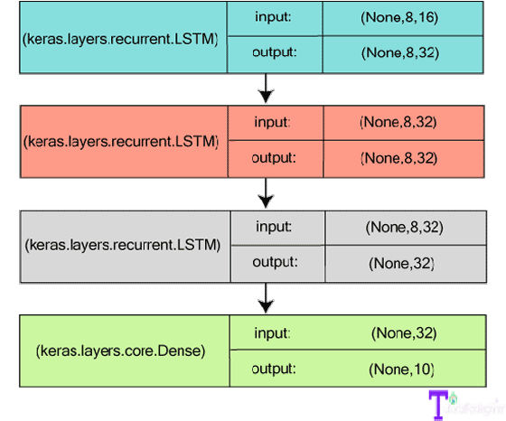
Stacked LSTM for Sequence Classification:
Three LSTM layers are stacked on top of one another to make the model capable of learning high-level temporal representation.
The layers are layered in such a way that the first two layers create complete output sequences and the third one provides the final phase in its output sequence, assisting in the successful translation of the input sequence to the single vector (i.e., dropdown of temporal dimension).
    from keras.models import Sequential
    from keras.layers import LSTM, Dense
    import numpy as np
    data_dim = 16
    timesteps = 8
    num_classes = 10

    #expected input data shape: (batch_size, timesteps, data_dim)
    model = Sequential ()
    model.add(LSTM(32, return_sequences=True,
                   input_shape(timesteps, data_dim))) #returns a sequence of sequence of vectors of dimension 32
    model.add(LSTM(32, return_sequences=True)) #returns a sequence of vectors of dimension 32
    model.add(LSTM(32)) #return a single vector of dimension 32
    model.add(Dense(10, activation='softmax'))
    model.compile(loss='categorical_crossentropy',
                  optimizer='rmsprop',
                  metrics=['accuracy'])

    #generate dummy training data
    x_train = np.random.random((1000, timesteps, data_dim))
    y_train = np.random.random((1000, num_classes))

    #generate dummy validation data
    x_val = np.random.random((100, timesteps, data_dim))
    y_val = np.random.random((100, num_classes))
    model.fit(x_train, y_train,
              batch_size=64, epochs=5,
              validation_data=(x_val, y_val))
Same Stacked LSTM model, rendered "stateful":
A "stateful recurrent model" is one whose central (internal) states are used as initial states for another batch of samples after a batch of samples has been processed. It not only manages computational complexity but also allows for the processing of longer sequences.
    from keras.models import Sequential
    from keras.layers import LSTM, Dense
    import numpy as np
    data_dim = 16
    timesteps = 8
    num_classes = 10
    batch_size = 32

    # Expected input batch shape: (batch_size, timesteps, data_dim)
    # Note that we have to provide the full batch_input_shape since the network is stateful.
    # the sample of index i in batch k is the follow-up for the sample i in batch k-1.

    model = Sequential()
    model.add(LSTM(32, return_sequences=True, stateful=True,
                   batch_input_shape=(batch_size, timesteps, data_dim)))
    model.add(LSTM(32, return_sequences=True, stateful=True))
    model.add(LSTM(32, stateful=True))
    model.add(Dense(10, activation='softmax'))

    model.compile(loss='categorical_crossentropy',
                  optimizer='rmsprop',
                  metrics=['accuracy'])

    # Generate dummy training data
    x_train = np.random.random((batch_size * 10, timesteps, data_dim))
    y_train = np.random.random((batch_size * 10, num_classes))

    # Generate dummy validation data
    x_val = np.random.random((batch_size * 3, timesteps, data_dim))
    y_val = np.random.random((batch_size * 3, num_classes))

    model.fit(x_train, y_train,
              batch_size=batch_size, epochs=5, shuffle=False,
              validation_data=(x_val, y_val))
Keras Functional API
The Keras Functional API is used to define sophisticated models such as multi-output models, directed acyclic models, and graphs with shared layers. In other words, the functional API allows you to outline the inputs and outputs that share layers.
First Example: A densely-connected network
The sequential model produces better results when implementing a densely connected network, although it would not be a terrible idea to experiment with another model.
The Keras Functional API implementation is comparable to the Keras Sequential Model implementation.
- A tensor invokes an instance layer, which returns a tensor as an output.
- Both input and output tensors are utilized to define a model.
    from keras.layers import Input, Dense
    from keras.models import Model
    # Returns a Tensor
    inputs = Input(shape=(784,))

    # An instance layer is callable on a tensor and returns a tensor
    output_1 = Dense(64, activation='relu')(inputs)
    output_2 = Dense(64, activation='relu')(output_1)
    predictions = Dense(10, activation='softmax')(output_2)

    # Creates a model that includes the Input layer and three Dense layers
    model = Model(inputs=inputs, outputs=predictions)
    model.compile(optimizer='rmsprop',
                loss='categorical_crossentropy',
                metrics=['accuracy'])
    model.fit(data, labels)  # start training
All models are callable, just like layers
Because we're talking about the functional API model, we can easily reuse the trained models by considering any such model as if it were a layer. It is accomplished by invoking a model on a tensor.
When we call a model on tenor, we are not only reusing its architecture but also its weights.
    x = Input(shape=(784,))
    # It works, and returns the 10-way softmax we defined above.
    y = model(x)
The code provided above enables an instance to construct a model for processing input sequences. We can also turn an image classification model into a video classification model using a single line.
    from keras.layers import TimeDistributed

    # Input tensor for sequences of 20 timesteps, such that each contains a 784-dimensional vector
    input_sequences = Input(shape=(20, 784))

    # It applies our previous model to every timestep in the input sequences. The output of the previous model was a 10-way softmax, so the output of the layer given below will be a sequence of 20 vectors of size 10.
    processed_sequences = TimeDistributed(model)(input_sequences)
Multi-input and multi-output models
Because a functional API explains multi-input and multi-output models well, it can manipulate a huge number of interwoven datastreams. Let's have a look at an example to get a better understanding of the subject. Essentially, we will anticipate how many retweets and likes a news headline will receive on social media platforms such as Twitter.
Both the headline, which is a sequence of words, and an auxiliary input, such as the time or date the headline was posted, will be sent to the model that accepts data. The two-loss functions are also used to supervise the model, so using the primary loss function in the first steps is the ideal choice for regularizing deep learning models.
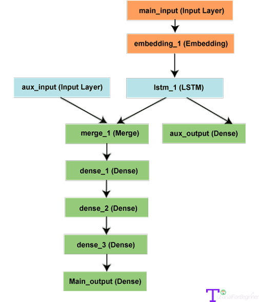
The main_input is obtained here as a sequence of integers, with each integer encoding one word. The integers run from 1 to 10,000, and the sequences are 100 words long.
    from keras.layers import Input, Embedding, LSTM, Dense
    from keras.models import Model
    import numpy as np
    np.random.seed(0)  # Sets a random seed for reproducibility.

    # Headline input receive sequences of 100 integers in between 1 and 10000.
    # Here we can name any layer by passing it a "name" argument.
    main_input = Input(shape=(100,), dtype='int32', name='main_input')

    # The embedding layer encodes the input sequence into a sequence of dense 512-dimensional vectors.
    x = Embedding(output_dim=512, input_dim=10000, input_length=100)(main_input)

    # The LSTM transforms the vector sequence into a single vector that contains the information about an entire sequence.
    lstm_out = LSTM(32)(x)
The auxiliary loss will then be introduced, allowing the LSTM and embedding layers to train smoothly even when the primary loss in the model is larger.
auxiliary_output = Dense(1, activation='sigmoid', name='aux_output')(lstm_out)
Next, we'll add the aux_input to our model by concatenating it with the LSTM output.
    auxiliary_input = Input(shape=(5,), name='aux_input')
    x = keras.layers.concatenate([lstm_out, auxiliary_input])

    # Stacks a densely-connected deep network on the top.
    x = Dense(64, activation='relu')(x)
    x = Dense(64, activation='relu')(x)
    x = Dense(64, activation='relu')(x)

    # Then add the main logistic regression layer.
    main_output = Dense(1, activation='sigmoid', name='main_output')(x)
    # Defines a model with two inputs and outputs
    model = Model(inputs=[main_input, auxiliary_input], outputs=[main_output, auxiliary_output])
Following that, we will construct our model by assigning a weight of 0.2 to the auxiliary loss. Then, for each separate output, we will utilize a list or a directory to identify the loss or loss_weight. A single loss parameter (loss) will be given to utilize the same loss on all outputs.
    model.compile(optimizer='rmsprop', loss='binary_crossentropy',
                  loss_weights=[1., 0.2])
Following that, we will train our model by sending lists of input and target arrays.
    headline_data = np.round(np.abs(np.random.rand(12, 100) * 100))
    additional_data = np.random.randn(12, 5)
    headline_labels = np.random.randn(12, 1)
    additional_labels = np.random.randn(12, 1)
    model.fit([headline_data, additional_data], [headline_labels, additional_labels],
               epochs=50, batch_size=32)
The model will be constructed as follows, based on the names we assigned to its inputs and outputs:
    model.compile(optimizer='rmsprop',
                  loss={'main_output': 'binary_crossentropy', 'aux_output': 'binary_crossentropy'},
                  loss_weights={'main_output': 1., 'aux_output': 0.2})

    # And train it through:
    model.fit({'main_input': headline_data, 'aux_input': additional_data},
              {'main_output': headline_labels, 'aux_output': additional_labels},
              epochs=50, batch_size=32)
The model can be inferenced by;
model.predict({'main_input': headline_data, 'aux_input': additional_data})
or,
pred = model.predict([headline_data, additional_data])
Shared layers:
The shared layers are another example to examine while understanding the functional API concept. We shall examine the tweet's dataset for this purpose. Because we are willing to create a model that can determine whether two tweets belong to the same person or not, it will be simple for an example to compare users based on tweet similarities.
We will build a model that will encode two tweets into vectors, concatenate them, and then add logistic regression. The model will generate a probability for two tweets from the same individual. Following that, we will train our model on pairs of both good and negative tweets.
Because our problem is symmetric in this case, our mechanism must reuse the first encoded tweet to encode the second tweet, for which we will use a shared LSTM layer.
We will input a binary matrix of shape (280, 256) for a tweet to build this model with a functional API. In this case, 280 is a 256-dimensional vector sequence that encodes the presence or absence of a character.
    import keras
    from keras.layers import Input, LSTM, Dense
    from keras.models import Model

    tweet_a = Input(shape=(280, 256))
    tweet_b = Input(shape=(280, 256))
Next, we will input a layer and then call it on various inputs as needed, allowing us to share a layer across multiple inputs.
    # The layer takes an input as a matrix and will return a vector of size 64
    shared_lstm = LSTM(64)

    # When we reuse the same layer instance multiple times, the weights of the layer will also be reused (it is effectively *the same* layer)
    encoded_a = shared_lstm(tweet_a)
    encoded_b = shared_lstm(tweet_b)

    # Next we will concatenate the two vectors:
    merged_vector = keras.layers.concatenate([encoded_a, encoded_b], axis=-1)

    # And then we will add logistic regression on top
    predictions = Dense(1, activation='sigmoid')(merged_vector)

    # After that we will define a trainable model by linking the tweet inputs to the predictions
    model = Model(inputs=[tweet_a, tweet_b], outputs=predictions)

    model.compile(optimizer='rmsprop',
                  loss='binary_crossentropy',
                  metrics=['accuracy'])
    model.fit([data_a, data_b], labels, epochs=10)
To understand how to read the shared layer's output or output shape, we'll take a quick look at the layer the concept of layer "node" notion.
When we call a layer on any input, we are creating a new tensor by appending a node to the layer and connecting the input tensors to the output tensor. If the same layer is called many times, it will own a certain number of nodes, which will be indexed as 0, 1, 2,...
In prior versions of Keras, we used layer.get_output() to get a layer instance's tensor output and layer.output_shape to get its output shape. However, get output() has now been replaced by output.
As long as one layer is coupled to a single input, the layer will return one output.
    a = Input(shape=(280, 256))

    lstm = LSTM(32)
    encoded_a = lstm(a)

    assert lstm.output == encoded_a
In the event that the layer has many inputs,
    a = Input(shape=(280, 256))
    b = Input(shape=(280, 256))

    lstm = LSTM(32)
    encoded_a = lstm(a)
    encoded_b = lstm(b)

    lstm.output
Output:
    >> AttributeError: Layer lstm_1 has multiple inbound nodes,
    hence the notion of "layer output" is ill-defined.
    Use `get_output_at(node_index)` instead.
It will now be carried out as follows:
    assert lstm.get_output_at(0) == encoded_a
    assert lstm.get_output_at(1) == encoded_b
The same is true for characters like input_shape and output_shape. Only when a layer consists of individual layers or all nodes with similar input and output can we conclude that the concept of "layer input and output shape" is fully defined and the shape will be returned by the layer. output shape or layer. input shape.
If we apply a conv2D layer to an input of forms (32, 32, 3) and subsequently to (64, 64, 3), the layer will contain numerous input/output shapes. And in order to retrieve them, we must give the index of nodes to which they belong.
    a = Input(shape=(32, 32, 3))
    b = Input(shape=(64, 64, 3))

    conv = Conv2D(16, (3, 3), padding='same')
    conved_a = conv(a)

    # Only one input so far, the following will work:
    assert conv.input_shape == (None, 32, 32, 3)

    conved_b = conv(b)
    # now the "input_shape" property wouldn't work, but this does:
    assert conv.get_input_shape_at(0) == (None, 32, 32, 3)
    assert conv.get_input_shape_at(1) == (None, 64, 64, 3)