Mini-max Algorithm in AI
Table of Content:
- What is the Mini-max Algorithm in Artificial Intelligence?
- How the Minimax algorithm works.
- Pseudo-code for MinMax Algorithm.
- Working of Min-Max Algorithm.
- Properties of Mini-Max algorithm.
- Limitation of the minimax Algorithm.
Content Highlight:
The Mini-Max algorithm in AI is fundamental for optimizing decisions in two-player, zero-sum games like chess. It aims to maximize the AI player's gain while minimizing the opponent's loss. Despite its effectiveness, Mini-Max relies on optimal play assumptions and faces complexity challenges in larger game trees.
What is the Mini-max Algorithm in Artificial Intelligence?
The Minimax algorithm is a fundamental concept in artificial intelligence, particularly in game theory and decision-making processes. It's commonly used in two-player, zero-sum games, where one player's gain is the other player's loss (e.g., chess, checkers, tic-tac-toe).
At its core, the Minimax algorithm is a way for an AI agent to make decisions by considering the possible outcomes of its own actions and its opponent's counter-actions, ultimately aiming to maximize its own advantage while minimizing the potential gain of the opponent.
The name "Minimax" comes from the strategy of minimizing the potential loss (for the opponent) while maximizing the potential gain (for the AI player). It operates on the principle of adversarial search, where the AI agent simulates the opponent's moves and chooses its own actions accordingly.
Although the Minimax algorithm is conceptually simple, its efficiency depends on the branching factor of the game tree and the depth to which it explores. In practice, optimizations like alpha-beta pruning are often used to reduce the search space and improve performance, especially in complex games with large branching factors.
How the Minimax algorithm works:
- Game Tree Generation: The algorithm begins by generating a game tree that represents all possible moves and counter-moves for both players, extending up to a certain depth or until a terminal state is reached.
- Evaluation Function: At the terminal nodes of the game tree (i.e., states where the game ends), an evaluation function is applied to determine the value of that state. This function assigns a score to the state based on how favorable it is for the player. For example, in chess, the evaluation function might consider factors like material advantage, piece positioning, and king safety.
- Recursion (Backtracking): Starting from the current game state, the algorithm recursively evaluates the possible moves, alternating between maximizing the AI player's score and minimizing the opponent's score. This recursion continues until a terminal node is reached (either the end of the game or a specified depth limit).
- Backtracking (Backpropagation): The algorithm then backtracks through the tree from the terminal nodes to the root, propagating the values of the terminal states upward. At each level, it alternates between maximizing (for the AI player) and minimizing (for the opponent player) the evaluated scores.
- Decision Making: Once the entire tree is evaluated, the AI agent selects the move that leads to the highest evaluated score assuming the opponent will also make optimal moves (i.e., it maximizes its potential gain while considering the opponent's potential counter-moves).
- Optimizations:: To improve performance and reduce computational overhead, various optimizations can be applied to the Minimax algorithm. One common optimization is alpha-beta pruning, which eliminates branches of the game tree that are guaranteed to be worse than previously evaluated branches, reducing the search space and improving efficiency.
Pseudo-code for MinMax Algorithm:
    function minimax(node, depth, maximizingPlayer) is
        if depth == 0 or node is a terminal node then
            return static evaluation of node

        if maximizingPlayer then      // for Maximizer Player
            maxEval = -infinity
            for each child of node do
                eval = minimax(child, depth - 1, false)
                maxEval = max(maxEval, eval)        //gives Maximum of the values
            return maxEval

        else                         // for Minimizer player
            minEval = +infinity
            for each child of node do
                eval = minimax(child, depth - 1, true)
                minEval = min(minEval, eval)         //gives minimum of the values
            return minEval
Initial call: minimax(node, 3, true)
Working of Min-Max Algorithm:
- Start with the initial game state and set the depth limit to 3.
- Assume the AI player is the Maximizer and wants to maximize its score.
- Consider the game tree representing possible moves and counter-moves for both players.
- Apply a depth-first search (DFS) approach to explore the tree.
- At each terminal node, assign values representing the outcome of the game.
- Backtrack through the tree, comparing the terminal values and selecting the best moves.
- If the Maximizer is the current player, choose the move with the highest value.
- If the Minimizer is the current player, choose the move with the lowest value.
- Continue backtracking until reaching the initial state.
- Return the selected move, which represents the best decision for the AI player.
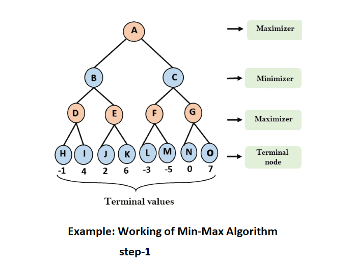
Step 1: In the first step, the algorithm generates the entire game tree and applies the utility function to obtain the utility values for the terminal states. In the below tree diagram, let's designate A as the initial state of the tree. Suppose the maximizer takes the first turn, which initializes with a worst-case initial value of -∞ or value =- ∞, and the minimizer will take the next turn, initialized with a worst-case initial value of +∞ or value = +∞.
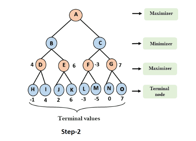
Step 2: Now, we begin by determining the utility values for the Maximizer. With an initial value of -∞, we compare each value in the terminal states with the Maximizer's initial value, selecting the highest value encountered. This process ensures that the Maximizer evaluates the tree nodes to find the maximum utility among them.
- For node D max(-1,- -∞) => max(-1,4)= 4
- For Node E max(2, -∞) => max(2, 6)= 6
- For Node F max(-3, -∞) => max(-3,-5) = -3
- For node G max(0, -∞) = max(0, 7) = 7
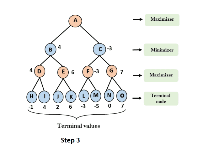
Step 3: In the next step, it's the turn for the Minimizer. It will compare all node values with +∞ and find the values of the nodes at the third layer.
- For node B = min(4,6) = 4
- For node C = min (-3, 7) = -3
In the next step, algorithm traverse the next successor of Node B which is node E, and the values of α = -∞, and β = 3 will also be passed.
Step 4: Now it's the turn for the Maximizer, and it will once again select the maximum of all node values to find the maximum value for the root node. In this game tree, there are only 4 layers, hence we reach immediately to the root node, but in real games, there will be more than 4 layers.
- For node A max(4, -3)= 4
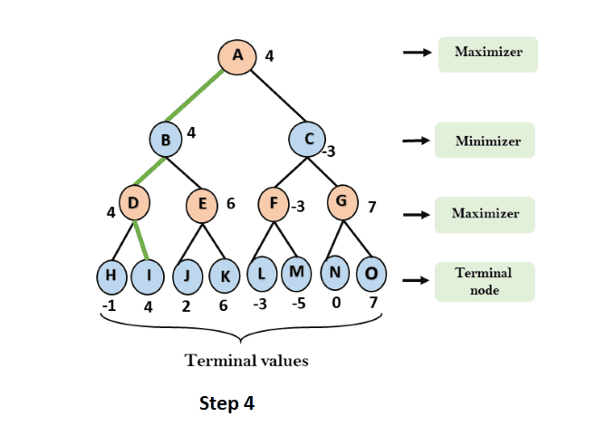
That was the complete workflow of the minimax two player game.
Properties of Mini-Max algorithm:
- Completeness: The Minimax algorithm is complete. It guarantees to find a solution (if one exists) within the finite search tree. This means that it will explore all possible paths in the game tree until it reaches a terminal state.
- Optimality: The Minimax algorithm is optimal when both opponents are playing optimally. This means that it will select moves that maximize the AI player's chances of winning while minimizing the opponent's chances, assuming both players make the best possible moves.
- Time Complexity: The time complexity of the Minimax algorithm is determined by the depth-first search (DFS) it performs on the game tree. It is represented as O(bm) , where b is the branching factor of the game tree (i.e., the average number of possible moves per state), and m is the maximum depth of the tree (i.e., the length of the longest path from the root to a leaf).
- Space Complexity: The space complexity of the Minimax algorithm is also similar to DFS, given by O(bm). It represents the amount of memory required to store the nodes and states explored during the search process. As the algorithm explores deeper into the tree, more memory is required to store the nodes at each level.
Limitation of the minimax Algorithm:
- Complexity: The Minimax algorithm struggles with large search spaces, leading to exponential time and space complexity as the depth of the game tree increases.
- Incomplete/Imperfect Information: The algorithm assumes perfect information and complete knowledge of the game state, which may not be realistic in games with incomplete or uncertain information.
- Optimality Assumption: Minimax assumes that both players will play optimally, which may not always hold true in real-world scenarios where human players may not make optimal decisions.
These limitations underscore the challenges and constraints faced by the Minimax algorithm in practical applications, particularly in complex games with large search spaces or imperfect information.