Uninformed search in AI
Table of Content:
- What is uninformed search in artificial intelligence?
- Breadth-first Search
- Depth-first Search
- Depth-Limited Search Algorithm
- Iterative deepening depth-first search
- Uniform cost search
- Bidirectional Search
Content Highlight:
Uninformed search in artificial intelligence refers to search algorithms that navigate a search space without additional information, relying on brute-force exploration. Examples include Breadth-First Search, Depth-First Search, Depth-Limited Search, Iterative Deepening Depth-First Search, Uniform-Cost Search, and Bidirectional Search. These algorithms have advantages such as completeness and simplicity but may face challenges like high memory requirements or suboptimal solutions, depending on the problem characteristics.
What is uninformed search in artificial intelligence?
Uninformed search represents a class of versatile search algorithms that navigate through a search space in a straightforward and brute-force manner. In the realm of uninformed search, algorithms lack any additional information about the states or structure of the search space, relying solely on their ability to traverse the exploration tree. This characteristic leads to the classification of these algorithms as blind searches.
In the domain of uninformed search, the absence of extra insights into the nature of the search space means that these algorithms embark on their exploration without any knowledge beyond the basic tree traversal mechanisms. Despite the seemingly simplistic approach, uninformed search algorithms play a vital role in various problem-solving scenarios. Their reliance on brute-force exploration makes them well-suited for tasks where an exhaustive examination of possibilities is essential.
The various types of uninformed search algorithms are as follows:
- Breadth-first Search
- Depth-first Search
- Depth-limited Search
- Iterative deepening depth-first search
- Uniform cost search
- Bidirectional Search
1. Breadth-first Search:
Breadth-first search (BFS) is a graph traversal algorithm meticulously designed to systematically explore and visit all vertices of a graph in a layer-by-layer fashion. Imagine a graph as a network of interconnected nodes, where each node represents a point of interest, and edges denote the relationships between them. Starting from a specified source node, BFS systematically explores the immediate neighbors of that node before moving on to their neighbors.
The algorithm uses a queue to keep track of the order in which vertices are discovered and visited. This ensures that BFS explores the graph level by level, making it particularly useful for finding the shortest path between two nodes in an unweighted graph. The key steps involve enqueueing the starting node, marking it as visited, dequeuing nodes for exploration, and enqueuing their unvisited neighbors until the entire graph is traversed. Breadth-first search is valuable in various applications, such as network routing, social network analysis, and puzzle solving, where understanding relationships and uncovering the shortest path are crucial.
A FIFO queue data structure was used to implement a breadth-first search.
An example of BFS:
In the following tree structure, the traversal of the tree using the BFS algorithm from the root node S to the goal node K is illustrated. BFS search algorithm explores the tree in layers, adhering to the path indicated by the dotted arrow. The traversed path is determined by this layer-by-layer exploration, ensuring a systematic and exhaustive search from the root to the goal.
S -→ A-→ B -→ C -→ D -→ G -→ H -→ E-→ F-→ I-→ K

Time Complexity: The number of nodes traversed in BFS till the shallowest Node can be used to determine the algorithm's time complexity. Where d represents the depth of the shallowest solution and b represents a node at each state.
Space Complexity: Space complexity of BFS algorithm is given by the Memory size of frontier which is O(bd).
T (b) = 1 + b2 + b3 + ... + bd = O(bd)
Completeness: BFS is complete, which means it will discover a solution if the shallowest target node is at a finite depth.
Optimality: BFS is optimal if the path cost is a non-decreasing function of the node's depth.
Advantages of Breadth-first Search:
- Shortest Path Finding: BFS guarantees finding the shortest path in an unweighted graph.
- Layer-by-Layer Exploration: BFS explores a graph in a layer-by-layer fashion, facilitating analysis of levels or layers.
- Connected Component Detection: It can be used to efficiently detect connected components in a graph.
- Algorithmic Simplicity: BFS is straightforward and easy to implement.
- Avoidance of Redundant Exploration: Marking visited nodes prevents redundant exploration and improves efficiency.
- Applications in Web Crawling: BFS is commonly used in web crawling algorithms for organized exploration of web pages.
- Applications in Puzzle Solving: Useful for solving puzzles and mazes, especially for finding optimal solutions.
- Applications in Network Routing: Plays a crucial role in determining efficient paths for data packets in network routing.
- Guaranteed Completeness: Ensures that all nodes in a connected graph are visited, providing completeness.
- Useful for Bipartite Graph Detection: Can be applied to determine if a graph is bipartite, with applications in various fields.
Disadvantages of Breadth-first Search:
- Memory Requirements: BFS may have higher memory requirements compared to other algorithms, especially when dealing with large graphs. This is because it needs to store information about all nodes at the current level.
- Time Complexity: In certain cases, BFS can have a higher time complexity compared to other search algorithms. It might explore unnecessary nodes, leading to inefficiencies.
- Suboptimal Solutions: While BFS guarantees the shortest path in unweighted graphs, it may find suboptimal solutions in weighted graphs, where the path with fewer edges might not be the path with the lowest total weight.
- Completeness for Infinite Graphs: BFS may not be suitable for infinite graphs as it continues to explore indefinitely. In such cases, it's not guaranteed to find a solution if one exists.
- Inefficiency in Dense Graphs: In dense graphs where the number of edges is close to the square of the number of vertices, BFS can be less efficient compared to other algorithms like DFS.
- Dependence on Initial Graph Representation: The way the graph is represented can impact the efficiency of BFS. For certain representations, such as an adjacency matrix, BFS may be less efficient.
2. Depth-first Search:
Depth-first Search (DFS) is a graph traversal algorithm that explores as far as possible along each branch before backtracking. Starting from a specified source node, DFS systematically visits the neighbors of the current node, diving deeper into the graph until it reaches a leaf node. If a dead-end is encountered, the algorithm backtracks to the nearest unexplored branch and continues the exploration.
DFS can be visualized as navigating through a maze by exploring one path until reaching an endpoint or a junction, then backtracking when needed. This algorithm is useful for tasks like maze solving, topological sorting, and detecting connected components in a graph.
An example of Depth-first Search:
The flow of depth-first search is depicted in the search tree below, and it will proceed in the following order:
Right node -→ root node -→ left node
It will begin its search from root node S and traverse A, B, D, and E; after traversing E, it will backtrack the tree because E has no successors and the goal node has yet to be discovered. It will retreat to node C and then to node G, where it will end because it has reached the goal node.

Completeness: Within a finite state space, the DFS search algorithm is complete since it expands every node within a constrained search tree.
Time Complexity: DFS's time complexity will be equal to the number of nodes traversed by the algorithm. It is provided by:
T(n)= 1+ n2+ n3 +.........+ nm = O(nm)
Where m is the greatest depth of any node, which can be significantly greater than d. (Shallowest solution depth)
Space Complexity: Because the DFS algorithm only has to record one path from the root node, its space complexity is equal to the size of the fringe set, which is O. (bm).
Optimal: DFS search algorithm is not optimum since it may result in a huge number of steps or a high cost to reach the goal node.
Advantage of Depth-first Search:
- Memory Efficiency: DFS typically requires less memory compared to Breadth-first Search (BFS) as it only needs to store information about the current branch being explored.
- Applications in Backtracking: DFS is well-suited for backtracking problems where exploring all possibilities is necessary, such as solving puzzles or searching for solutions.
- Useful for Pathfinding: In certain scenarios, DFS can be more efficient for pathfinding in mazes or networks with a large number of possible paths.
- Topological Sorting: DFS is commonly used for topological sorting in directed acyclic graphs, a crucial operation in scheduling and task planning.
- Applications in Game Trees: DFS is employed in game trees for decision-making processes, exploring potential moves and strategies in games like chess or tic-tac-toe.
- Compact Representation: DFS is suitable for representing and navigating through sparse graphs efficiently.
Disadvantage of Depth-first Search:
- Completeness: DFS may not guarantee finding the optimal solution in certain scenarios. It can get stuck in infinite loops or fail to find a solution if the search space is infinite.
- Non-Optimal for Shortest Path: DFS does not always find the shortest path between two nodes, as it may find a solution along a longer path before exploring shorter paths.
- Memory Usage: In graphs with deep paths or in cases of infinite-depth graphs, DFS can use a large amount of memory due to the recursion stack, leading to potential stack overflow issues.
- Dependence on Branching Factor: The efficiency of DFS can heavily depend on the branching factor of the graph. High branching factors can lead to increased memory usage and longer execution times.
- Not Suitable for Weighted Graphs: DFS is not designed to handle weighted graphs efficiently, and it may not always yield optimal solutions in such cases.
- Applications in Cyclic Graphs: In cyclic graphs, DFS may result in traversing the same nodes multiple times, potentially leading to inefficiencies.
3. Depth-Limited Search Algorithm:
A depth-limited search algorithm works similarly to a depth-first search but with a limit. The problem of the endless path in the Depth-first search can be overcome by depth-limited search. The node at the depth limit will be treated as if it has no additional successor nodes in this procedure.
Two conditions of failure can be used to end a depth-limited search:
- Standard Failure Value: This signals that the problem does not possess any solution.
- Cutoff Failure Value: This specifies that there is no solution for the problem within a given depth limit.
An example of depth-limited search:

Completeness: If the solution is above the depth-limit, the DLS search procedure is complete.
Time Complexity: The DLS algorithm has a time complexity of O(bℓ)
Space Complexity: The DLS algorithm has a space complexity of O(bℓ)
Depth-limited search can be considered a variant of DFS, and it remains non-optimal even when the depth limit ℓ exceeds the depth of the solution d.
Advantages of Depth-Limited Search:
- Efficient Memory Usage: Depth-Limited Search efficiently manages memory as it only stores information about nodes within the specified depth limit.
- Prevention of Endless Paths: Depth-Limited Search overcomes the issue of endless paths that can occur in traditional Depth-First Search by restricting the exploration depth.
- Resource Control: The algorithm allows for better control over computational resources by setting a depth limit, preventing excessive memory usage and infinite loops.
- Termination Conditions: Depth-Limited Search provides clear termination conditions, distinguishing between standard failure (indicating no solution) and cutoff failure (indicating no solution within the depth limit).
- Useful in Resource-Constrained Environments: This approach is particularly beneficial in resource-constrained environments where limiting the depth of exploration is crucial for efficient problem-solving.
- Adaptability to Limited Knowledge: Depth-Limited Search is adaptable to scenarios where only limited knowledge about the problem space is available, making it suitable for various applications.
Disadvantages of Depth-Limited Search:
- Risk of Missing Solutions: Depth-Limited Search may miss optimal solutions that lie beyond the specified depth limit, potentially overlooking better paths in the search space.
- Dependence on Depth Limit: The effectiveness of Depth-Limited Search heavily relies on choosing an appropriate depth limit. An inadequate limit may lead to inefficiencies or failure to find a solution.
- Doesn't Handle Infinite Paths: Like Depth-First Search, Depth-Limited Search cannot handle problems with infinite paths, as it may still get stuck in cycles or infinite loops within the set depth.
- Potential for Suboptimal Solutions: The algorithm might yield suboptimal solutions if the optimal path exceeds the depth limit, impacting its performance in certain scenarios.
- Sensitivity to Initial Settings: The outcome of Depth-Limited Search can be sensitive to the initial depth limit and may require adjustments based on the specific characteristics of the problem space.
- Not Suitable for All Problems: Depth-Limited Search is not universally applicable and may not be the best choice for problems where the optimal solution lies beyond the chosen depth limit.
4. Uniform-cost Search Algorithm:
Uniform-cost search is an essential algorithm utilized for exploring weighted trees or graphs, particularly when each edge carries a distinct cost. This algorithm becomes crucial in scenarios where the goal is to uncover a path to the destination node with the lowest cumulative cost. Operating by expanding nodes based on their individual path costs from the root node, uniform-cost search employs a priority queue. This prioritization ensures that nodes with the lowest cumulative cost receive maximum priority. Ideal for solving graphs or trees with varying edge costs, the uniform-cost search algorithm is versatile and in demand wherever an optimal cost solution is required. Notably, it shares similarities with the BFS algorithm when the path cost of all edges is uniform.
Time Complexity: Let C* be the cost of the optimal solution, and ε represent each step to approach the goal node. The number of steps is given by C*/ε + 1. Considering we start from state 0 and conclude at C*/ε, we include a +1.
Hence, the worst-case time complexity of Uniform-cost search is O(b1 + [C*/ε]).
Space Complexity: Applying the same logic, the worst-case space complexity of Uniform-cost search is O(b1 + [C*/ε]).
Optimal: Uniform-cost search is always optimal as it exclusively selects paths with the lowest path cost.
Advantages of Uniform-cost Search:
- Optimal Solutions: Uniform-cost search ensures the discovery of optimal solutions by prioritizing paths with the lowest cumulative cost, making it suitable for problems where minimizing cost is critical.
- Adaptability to Varied Edge Costs: The algorithm is versatile and can handle scenarios with different costs associated with each edge, making it applicable to a wide range of problems.
- Exploration of All Possible Paths: Uniform-cost search systematically explores paths from the root node, providing a comprehensive analysis of potential solutions and guaranteeing an exhaustive search for the optimal one.
- Effective Implementation with Priority Queue: Implemented using a priority queue, the algorithm efficiently manages and prioritizes nodes based on their cumulative costs, contributing to its effectiveness in finding optimal solutions.
- Applicability to Any Graph or Tree: Uniform-cost search can be applied to solve any graph or tree where the demand for an optimal cost solution exists, showcasing its broad applicability.
- Consistency with BFS for Uniform Edge Costs: When the path cost of all edges is the same, uniform-cost search aligns with BFS, providing consistency and adaptability in different scenarios.
Disadvantages of Uniform-cost Search:
- Computational Complexity: Uniform-cost search can become computationally expensive, particularly in scenarios with large graphs or when dealing with varied and high edge costs.
- Memory Requirements: The algorithm may demand significant memory resources, especially when exploring paths with diverse cumulative costs, potentially leading to memory constraints in certain situations.
- Dependency on Edge Cost Information: Uniform-cost search heavily relies on accurate information about edge costs. Inaccurate or incomplete cost data can lead to suboptimal or incorrect solutions.
- Inefficiency in the Presence of Uniform Edge Costs: In cases where the path cost of all edges is uniform, uniform-cost search may exhibit inefficiencies, as it becomes equivalent to BFS without utilizing its priority queue advantage.
- Not Ideal for Some Applications: While effective for optimal pathfinding, uniform-cost search may not be the best choice for problems where minimizing cost is not a primary consideration.
- Sensitivity to Graph Structure: The efficiency of uniform-cost search can be sensitive to the structure of the graph, and certain graph configurations may impact its performance negatively.
5. Iterative deepening depth-first Search:
The iterative deepening algorithm cleverly blends the characteristics of both DFS and BFS. This search algorithm identifies the optimal depth limit by progressively increasing it until reaching the goal.
It executes a depth-first search within a defined "depth limit" and iteratively elevates this limit until the goal node is successfully located. The iterative search algorithm strategically combines the speedy search capabilities of Breadth-first search with the memory efficiency of depth-first search.
This algorithm proves particularly beneficial in uninformed searches when dealing with extensive search spaces, and the depth of the goal node remains unknown.
The iterative deepening depth-first search is demonstrated in the following tree structure. The IDDFS algorithm iterates until it can't find the goal node any longer. The algorithm's iteration is described as follows:
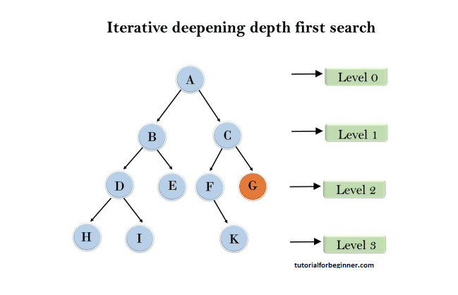
1'st Iteration ⇒ A
2'nd Iteration ⇒ A, B, C
3'rd Iteration ⇒ A, B, D, E, C, F, G
4'th Iteration ⇒ A, B, D, H, I, E, C, F, K, G
In the fourth iteration, the algorithm will find the goal node.
Completeness: If the branching factor is finite, this algorithm is complete.
Time Complexity: If the branching factor is b and the depth is d, the worst-case time complexity is O(bd).
Space Complexity: IDDFS will have an O space complexity (bd).
Optimal: If path cost is a non-decreasing function of node depth, the IDDFS algorithm is optimal.
Advantages of Iterative deepening depth-first:
- Optimal Solution: Iterative Deepening Depth-First Search guarantees finding an optimal solution, ensuring that it explores the shortest path to the goal node.
- Memory Efficiency: It combines the memory efficiency of Depth-First Search, only storing information about the current branch, with the systematic search approach, preventing excessive memory usage.
- Adaptability to Unknown Depths: Well-suited for scenarios where the depth of the goal node is unknown, as it incrementally increases the depth limit until a solution is found.
- Effective for Large Search Spaces: Particularly useful in searches involving large search spaces where a balance between memory efficiency and exploration depth is crucial.
- Gradual Exploration: It performs a gradual exploration, focusing on shallow depths first before moving deeper, providing a balance between Breadth-First and Depth-First Search strategies.
- Usefulness in Uninformed Searches: Valuable in uninformed searches when little prior knowledge about the search space is available, making it versatile for various applications.
Disadvantages of Iterative deepening depth-first:
- Repetitive Exploration: Iterative Deepening Depth-First Search may redundantly explore nodes at various depth levels, potentially leading to inefficient exploration in certain scenarios.
- Redundant Work: The algorithm performs redundant work by revisiting nodes at shallower depths in each iteration, which could impact its efficiency, especially in cases where exploration beyond a certain depth is unnecessary.
- Dependency on Goal Depth: The effectiveness of the algorithm relies on a reasonable estimation of the goal depth, and incorrect assumptions may result in suboptimal performance or failure to find a solution.
- Not Suitable for All Problems: While advantageous in certain scenarios, Iterative Deepening Depth-First Search may not be the most suitable approach for problems where a known depth limit or extensive knowledge about the search space is available.
- Increased Overhead: The iterative nature of the algorithm introduces additional overhead in terms of repeated searches at varying depth levels, potentially impacting its time complexity.
- Less Efficient for Uniform Edge Costs: In scenarios where edge costs are uniform, the algorithm may exhibit less efficiency compared to other search strategies, as it converges towards Breadth-First Search.
6. Bidirectional Search Algorithm:
Bidirectional search algorithm operates by concurrently running two searches—forward-search from the initial state and backward-search from the goal node—in pursuit of finding the goal node. This approach replaces a single expansive search graph with two smaller subgraphs, each starting its exploration from either the initial or goal vertex. The algorithm concludes when these two subgraphs intersect, marking the discovery of the goal node.
Bidirectional search is versatile and can employ various search techniques like BFS, DFS, DLS, etc., enhancing its adaptability to different problem scenarios. This bidirectional strategy aims to streamline the search process by narrowing down the exploration space from both ends, ultimately converging on a common intersection point.
An example of bidirectional search:
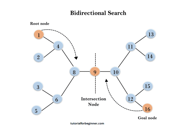
In the following search tree, the bidirectional search algorithm is employed. This innovative approach divides the original graph or tree into two distinct sub-graphs, initiating traversal from node 1 in the forward direction and simultaneously starting from the goal node 16 in the backward direction.
The bidirectional search algorithm efficiently explores both ends of the graph or tree, converging towards a common point. In this particular scenario, the algorithm concludes its exploration at node 9, where the forward and backward searches meet, marking the termination point.
Completeness: If we utilize BFS in both searches, we have a full bidirectional search.
Time Complexity: The bidirectional search using BFS has a time complexity of O(bd).
Space Complexity: The bidirectional search has a space complexity of O(bd).
Optimal: Bidirectional search is Optimal.
Advantages of Bidirectional Search:
- Faster Exploration: Bidirectional Search often leads to faster exploration compared to traditional search algorithms, as it converges from both the initial and goal states simultaneously.
- Reduced Search Space: By exploring from both ends, bidirectional search significantly reduces the overall search space, optimizing the search process and enhancing efficiency.
- Optimal Solutions: The algorithm tends to find optimal solutions, particularly in scenarios where the search space is well-defined and the optimal path is sought.
- Enhanced Memory Efficiency: Bidirectional Search exhibits improved memory efficiency as it explores smaller subgraphs from both directions, minimizing the storage requirements compared to exhaustive single-direction searches.
- Applicability to Large Graphs: Particularly useful for large graphs, bidirectional search provides a practical approach to efficiently navigate complex structures and identify goal nodes.
- Adaptability to Various Search Techniques: Bidirectional Search can accommodate different search techniques such as BFS, DFS, or DLS, making it versatile and suitable for diverse problem-solving scenarios.
Disadvantages of Bidirectional Search:
- Complex Implementation: Bidirectional Search can involve complex implementation compared to traditional search algorithms, requiring careful synchronization of forward and backward searches.
- Dependency on Accurate Heuristics: The effectiveness of bidirectional search may heavily depend on the availability of accurate heuristics, and suboptimal heuristics could lead to less efficient exploration.
- Sensitivity to Initial Graph Conditions: The performance of bidirectional search can be sensitive to the initial conditions of the graph, and certain graph configurations may impact its efficiency negatively.
- Not Ideal for All Problems: While advantageous in certain scenarios, bidirectional search may not be the most suitable approach for problems where the optimal solution is not a primary consideration.
- Increased Overhead: Managing two simultaneous searches introduces additional overhead, potentially impacting the overall time complexity of the bidirectional search algorithm.
- Application Complexity: Implementing bidirectional search in certain applications may introduce additional complexity, requiring careful consideration of the problem structure and search space.