Classification Algorithms in ML
Table of Contents:
- What is a Classification Algorithm?
- How Classification Algorithms Work
- Binary Classifiers
- Multi-Class Classifiers
- Types of Learners in Classification Problems
- Types of Classification Models
- Evaluating Classification Models
- Real-World Applications of Classification Algorithms
- Conclusion
Content Highlight:
This guide provides a concise overview of classification algorithms in supervised machine learning, covering binary and multi-class classifiers, how they work, and their applications in tasks like spam detection and speech recognition. It highlights key types of models, including Logistic Regression, SVM, and Random Forests, with Python implementation examples. Evaluation metrics like accuracy, precision, recall, F1 score, and AUC-ROC are explained for assessing performance. With practical examples, visuals, and code snippets, this guide simplifies understanding and applying classification algorithms effectively.
What is Classification Algorithm in Machine Learning?
The Classification Algorithm is a fundamental concept in Supervised Machine Learning, used to predict the category or class of new data points based on a labeled training dataset. In this technique, the model learns patterns from the input data along with their respective labels or classes and then uses these patterns to categorize new, unseen observations. Classification is widely applied in tasks where the output is discrete, such as binary classifications like "Yes" or "No," "Spam" or "Not Spam," and "Cat" or "Dog," as well as multiclass classifications, where an observation might belong to one of several possible classes.
Unlike regression algorithms, where the output variable is continuous (e.g., predicting sales or temperature), classification algorithms produce a categorical result. For example, instead of predicting a specific shade of color, a classification algorithm would categorize an item as "Red," "Green," or "Blue." Since classification is a supervised learning technique, it requires labeled data, meaning each input observation is paired with its correct output category, allowing the model to learn the relationship between input features and output classes.
How Classification Algorithms Work:
A classification model works by mapping input variables (x) to a discrete output variable (y) based on the function:
y = f(x)
Here, y is a categorical output representing the predicted class of the input data x. Through training, the model identifies boundaries or criteria that separate data points into distinct classes. For instance, in a dataset where features of email content are analyzed to detect spam, a classification algorithm learns to label emails as "Spam" or "Not Spam" based on past examples.
In the context of classification algorithms, the term classifier refers to the specific algorithm that applies the classification technique to a dataset. Classifiers fall into two primary categories:
1. Binary Classifier
A Binary Classifier is designed for classification tasks that yield only two possible outcomes, offering a straightforward and decisive result. This type of classifier distinguishes between two exclusive categories, allowing it to solve questions that require a clear “either-or” decision. Examples include:
- Yes or No (e.g., eligibility checks)
- Male or Female (gender classification)
- Spam or Not Spam (email categorization)
- Cat or Dog (basic image classification)
Binary classifiers are highly effective for tasks with clear-cut distinctions, optimizing performance in scenarios with mutually exclusive outcomes.
2. Multi-Class Classifier:
A Multi-Class Classifier addresses more complex scenarios where the classification involves more than two possible outcomes, often tackling broader categories and nuanced distinctions. This classifier can assign an observation to one of several classes, making it suitable for richly varied datasets. Examples include:
- Classification of Crop Types (e.g., identifying types of crops such as wheat, rice, or barley)
- Genre Classification in Music (e.g., categorizing music into genres like jazz, rock, or classical)
Multi-class classifiers are instrumental in fields where diverse categories are inherent to the data, requiring an adaptable approach to accommodate multiple outcomes.
Example: Email Spam Detector:
A practical example of a classification algorithm is an Email Spam Detector. This algorithm categorizes incoming emails as either "Spam" or "Not Spam." By analyzing the content, metadata, and sender information of emails, the model learns patterns indicative of spam. When applied to new emails, the model can automatically classify them, helping users avoid unwanted messages.
Goal of Classification Algorithms:
The main goal of classification algorithms is to accurately categorize or label data points based on their features. Classification is especially suited for problems where the output variable is categorical, and the focus is on determining which category or class a data point belongs to. These algorithms are used to predict outcomes, recognize patterns, and make informed decisions in diverse fields, from medical diagnoses and customer segmentation to financial fraud detection.
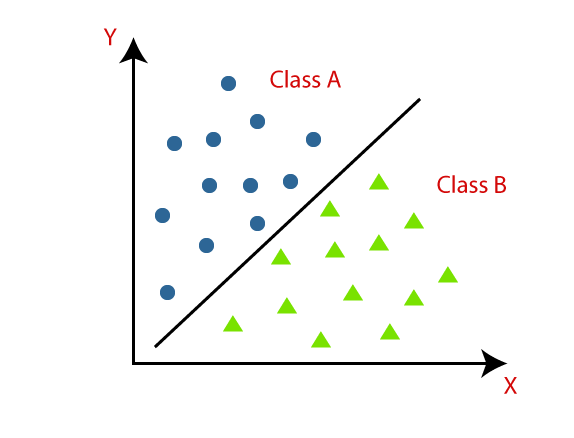
Visualizing Classification:
In the classification diagram, data points are grouped into two classes, Class A and Class B. Each class has distinct characteristics or features that distinguish it from the other. By recognizing these unique features, a classification model can effectively separate data into the appropriate categories, identifying shared attributes within each class while differentiating between classes.
This classification technique is a powerful tool for understanding and making decisions based on categorical data, providing valuable insights across a wide range of applications in machine learning.
Types of Learners in Classification Problems:
In classification problems, learners are the mechanisms or algorithms that interpret the data to make predictions. Classification learners fall into two primary categories, each with a unique approach to training and prediction processes.
Lazy Learners
Lazy Learners are those that delay the learning process until a test dataset or query is provided. Rather than building a general model from the training data, lazy learners retain the entire training set and perform minimal processing until a classification is required. This approach allows for flexibility and adaptation to new data since no fixed model is built initially. However, this flexibility comes at the cost of slower predictions, as the model must compute relationships from the training data on the fly for each new instance.
Characteristics:
- Training Speed: Very fast, as lazy learners do not build a model or analyze patterns during training.
- Prediction Speed: Slower, as the algorithm must search through the training data for similar instances to make predictions.
- Use Case: Ideal for smaller datasets or cases where training speed is more critical than prediction speed.
Examples:
- K-Nearest Neighbors (K-NN): This algorithm classifies a data point based on the majority class among its K closest points in the training set. It’s widely used in applications like recommendation systems and pattern recognition.
- Case-Based Reasoning: This method solves new problems by adapting solutions from similar past cases stored in the training data, commonly used in problem-solving and diagnostic systems.
Eager Learners:
Eager Learners take an opposite approach by constructing a classification model as soon as they receive the training data. This model learns and generalizes from the training examples, creating a fixed structure for decision-making. Eager learners invest more time and resources in analyzing data patterns upfront, resulting in faster predictions once a query is made. This type of learner is beneficial in applications where the prediction speed is essential.
Characteristics:
- Training Speed: Slower due to extensive model building and pattern extraction from the training data.
- Prediction Speed: Fast, as the model is pre-built and doesn’t require scanning the training dataset during prediction.
- Use Case: Suitable for larger datasets and scenarios requiring rapid prediction responses.
Examples:
- Decision Trees: Decision trees divide data into subsets based on attribute values, forming branches and leaves that represent decision points and outcomes. They are used in medical diagnoses, risk assessment, and customer segmentation.
- Naïve Bayes: A probabilistic classifier based on Bayes’ theorem, which assumes feature independence. Naïve Bayes is popular for text classification tasks, such as spam detection and sentiment analysis.
- Artificial Neural Networks (ANN): These consist of interconnected layers of nodes (neurons) that learn complex relationships in data, commonly used for image and speech recognition tasks.
Types of Machine Learning Classification Algorithms:
Classification algorithms can be organized into two primary categories, each featuring models that handle linear or non-linear decision boundaries.
1. Linear Models:
Linear models are effective for problems where data classes can be separated by a straight line (or hyperplane in higher dimensions). They are typically easier to interpret and train faster, making them ideal for simpler datasets.
- Logistic Regression: Despite its name, logistic regression is a classification algorithm that estimates the probability of a data point belonging to a particular class by applying the logistic function. It’s often used for binary classification tasks, such as customer churn prediction and medical diagnostics.
- Support Vector Machines (SVM): SVM finds the optimal hyperplane that separates classes in the dataset, maximizing the margin between the classes. SVM is widely applied in tasks like image classification, text categorization, and bioinformatics.
2. Non-Linear Models:
Non-linear models are better suited for complex datasets where the class boundaries are non-linear or curved. These algorithms allow for greater flexibility and adaptability in finding patterns within data.
- K-Nearest Neighbors (K-NN): As a lazy learner, K-NN uses the distances between points to classify new data based on its K nearest neighbors. It’s especially useful in recommendation systems, pattern recognition, and anomaly detection.
- Kernel Support Vector Machine (Kernel SVM): Kernel SVM extends the SVM approach to non-linearly separable data by transforming the original features into a higher-dimensional space. This method is commonly used in image processing and handwriting recognition.
- Naïve Bayes: This algorithm uses a simple probabilistic approach based on Bayes’ theorem, assuming independence between features. It performs particularly well in text analysis and spam filtering.
- Decision Tree Classification: Decision trees create a model that splits data into branches based on feature values, making it easy to interpret and visualize. They are applied in customer segmentation, credit risk assessment, and medical diagnostics.
- Random Forest Classification: An ensemble method that builds multiple decision trees and merges their outputs, enhancing accuracy and reducing overfitting. Random forests are versatile and are used in tasks like fraud detection, loan approval, and recommendation systems.
Evaluating a Classification Model:
After building a Classification Model, it’s vital to assess its accuracy and reliability. Evaluation metrics enable us to quantify how well the model performs in classifying new data points. Here are some of the most widely used evaluation methods:
1. Log Loss or Cross-Entropy Loss:
Log Loss or Cross-Entropy Loss is a measure of the accuracy of a classifier that provides probability-based predictions. Instead of just checking if a prediction is right or wrong, log loss evaluates how confident the model was in its predictions, penalizing predictions that are both wrong and confidently incorrect. Lower values of log loss indicate better performance.
- Ideal Value: For a well-performing binary classification model, log loss should be close to 0, indicating high predictive accuracy.
- Interpretation: The log loss increases as the predicted probability deviates from the actual class. This helps identify not just incorrect predictions but also how much the prediction deviated from reality.
- Formula for binary classification:
where:
- y is the actual label (1 for positive class, 0 for negative class),
- p is the predicted probability of the positive class.
In a multi-class setting, log loss can be extended to handle multiple classes by summing the individual losses for each class and then normalizing by the number of instances.
2. Confusion Matrix:
The Confusion Matrix is a tabular representation of the true classifications versus the predicted classifications. It provides a more detailed analysis by revealing not just the number of correct predictions, but also the types of errors. This matrix consists of four essential components:
- True Positives (TP): Cases where the model correctly predicted the positive class.
- False Positives (FP): Cases where the model incorrectly predicted the positive class when it was actually negative, also known as Type I error.
- True Negatives (TN): Cases where the model correctly predicted the negative class.
- False Negatives (FN): Cases where the model incorrectly predicted the negative class when it was actually positive, also known as Type II error.
Using these values, we can derive key performance metrics:
- Accuracy: Proportion of correctly predicted instances out of total predictions.
Accuracy = TP + TN TP + FP + TN + FN
- Precision: Proportion of positive predictions that are actually correct, helpful when false positives are costly.
Precision = TP TP+FP
- Recall (Sensitivity): Proportion of actual positives that are correctly predicted, crucial for detecting positives.
Recall = TP TP+FN
- F1 Score: Harmonic mean of precision and recall, useful for imbalanced datasets.
F1 Score = 2 X Precision × Recall Precision + Recall
The confusion matrix allows modelers to assess not just overall accuracy but also the types and rates of specific errors, leading to a more nuanced understanding of model performance.
3. AUC-ROC Curve:
The ROC Curve (Receiver Operating Characteristic Curve) is a graphical representation that showcases the performance of a classification model across various decision thresholds. The AUC (Area Under the Curve) value summarizes this performance; a value closer to 1 indicates a strong classifier.
- True Positive Rate (TPR), or Recall: Represents the proportion of actual positives correctly identified by the model. It is plotted on the Y-axis of the ROC curve.
TPR = TP TP + FN
- False Positive Rate (FPR): Represents the proportion of actual negatives that were incorrectly classified as positive. It is plotted on the X-axis of the ROC curve.
FPR = FP FP + TN
By adjusting the classification threshold, the model’s sensitivity and specificity can be balanced according to application requirements. A perfect classifier would have an AUC of 1, while a model performing no better than random guessing would have an AUC of 0.5.
Common Use Cases for Classification Algorithms:
Classification algorithms are essential tools for categorizing data into distinct classes, enabling decisions and actions across a variety of fields. Here are some prominent use cases:
- Email Spam Detection: Classifiers like Naïve Bayes or Logistic Regression distinguish between spam and legitimate emails based on email content and sender patterns, improving inbox management and security.
- Speech Recognition: Using algorithms like Hidden Markov Models (HMM) or Deep Neural Networks (DNN), speech recognition systems categorize audio signals into phonetic segments, which can then be converted to text. This technology powers virtual assistants, transcription services, and language learning tools.
- Cancer Tumor Identification: In medical imaging, Convolutional Neural Networks (CNNs) can identify and classify tumor cells from MRI or CT scans, assisting in early cancer detection and accurate diagnosis.
- Drug Classification: Algorithms such as Random Forests or Support Vector Machines (SVM) classify drugs based on chemical properties, structure, or pharmacological effects, aiding in pharmaceutical research and development.
- Biometric Identification: Classification models like k-Nearest Neighbors (K-NN) or Support Vector Machines help identify individuals based on unique physical characteristics, such as fingerprints, facial features, or retinal patterns. These models are crucial in security and access control systems.
Conclusion:
Classification algorithms are fundamental to decision-making across fields, and their impact continues to grow as advancements in machine learning and computational power make these methods more accurate, adaptable, and scalable. With careful evaluation, we can ensure these algorithms deliver precise, reliable results tailored to the specific needs of various applications.