Random Forest Algorithm in Machine Learning
In this page, we will learn What is Random Forest Algorithm?, Assumptions for Random Forest, Why use Random Forest?, How does Random Forest algorithm work?, Applications of Random Forest, Advantages of Random Forest, Disadvantages of Random Forest, Python Implementation of Random Forest Algorithm.
What is Random Forest Algorithm?
Random Forest is a well-known machine learning algorithm that
uses the supervised learning method. In machine learning, it
can be utilized for both classification and regression issues.
It is based on ensemble learning, which is a method of
integrating several classifiers to solve a complex problem and
increase the model's performance.
As the name suggests,
"Random Forest is a classifier that contains a number of
decision trees on various subsets of the given dataset and
takes the average to improve the predictive accuracy of that
dataset."
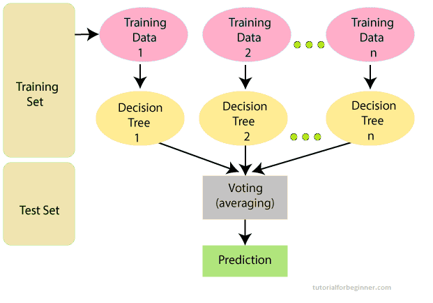
Instead than relying on a single decision tree, the random
forest collects the forecasts from each tree and predicts the
final output based on the majority votes of predictions.
The greater number of trees in the forest leads to higher
accuracy and prevents the problem of overfitting.
The below diagram explains the working of the Random Forest
algorithm:
Note: You need be familiar with the Decision Tree Algorithm in order to properly comprehend the Random Forest Algorithm.
Assumptions for Random Forest
Because the random forest combines numerous trees to forecast
the dataset's class, some decision trees may correctly predict
the output while others may not. However, when all of the
trees are combined, the proper result is predicted. As a
result, two assumptions for a better Random forest classifier
are as follows:
- The dataset's feature variable should have some actual values so that the classifier can predict accurate results rather than guesses.
- Each tree's predictions must have very low correlations.
Why use Random Forest?
The following are some reasons why we should utilize the Random Forest algorithm:
- When compared to other algorithms, it takes less time to train.
- It predicts output with good accuracy, and it runs quickly even with a huge dataset.
- When a considerable amount of the data is missing, it can still maintain accuracy.
How does Random Forest algorithm work?
The random forest is formed in two phases: the first is to
combine N decision trees to build the random forest, and the
second is to make predictions for each tree created in the
first phase.
The following steps and diagram can be used to demonstrate the
working process:
Step 1: Pick K data points at random from the training
set.
Step 2: Create decision trees for the data points
you've chosen (Subsets).
Step 3: Decide on the number N for the decision trees
you wish to create.
Step 4: Repetition of Steps 1 and 2.
Step 5: Find the forecasts of each decision tree for
new data points, and allocate the new data points to the
category with the most votes.
The following example will help you understand how the
algorithm works:
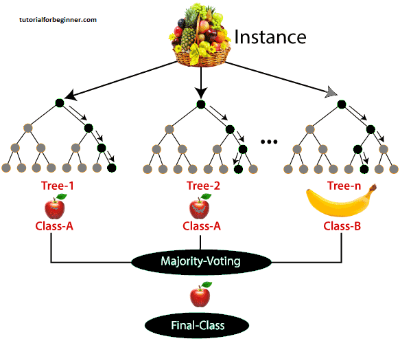
Example: There is a dataset including several fruit photos. As a result, the Random forest classifier is given this dataset. Each decision tree is given a portion of the dataset to work with. During the training phase, each decision tree generates a prediction result, and when a new data point appears, the Random Forest classifier predicts the final decision based on the majority of results. Consider the following illustration:
Applications of Random Forest
Random forest is most commonly utilized in the following four sectors:
- Banking: This algorithm is mostly used in the banking industry to identify loan risk.
- Medicine: This method can be used to identify disease trends as well as disease risks.
- Land Use: Using this technique, we can find places with comparable land use.
- Marketing: This algorithm can be used to identify marketing trends.
Advantages of Random Forest
- Random Forest can handle both classification and regression problems.
- It can handle huge datasets with a lot of dimensionality.
- It improves the model's accuracy and eliminates the problem of overfitting.
Disadvantages of Random Forest
- Despite the fact that random forest may be used for both classification and regression problems, it is not better suited to regression.
Python Implementation of Random Forest Algorithm
Now we'll use Python to implement the Random Forest Algorithm
tree. We'll use the same dataset "user data.csv" that we did
in prior classification models for this. We may compare the
Random Forest classifier against other classification models
such as Decision Tree Classifier, KNN, SVM, Logistic
Regression, and others using the same dataset.
Implementation Steps are given below:
- Data Pre-processing step
- Fitting the Random forest algorithm to the Training set
- Predicting the test result
- Test accuracy of the result (Creation of Confusion matrix)
- Visualizing the test set result.
1. Data Pre-Processing Step:
Below is the code for the pre-processing step:
   #importing libraries
   import numpy as nm
   import matplotlib.pyplot as mtp
   import pandas as pd

   #importing datasets
   data_set = pd.read_csv('user_data.csv')

   #Extracting Independent and dependent Variable
   x = data_set.iloc[:, [2,3]].values
   y = data_set.iloc[:, 4].values

   # Splitting the dataset into training and test set.
   from sklearn.model_selection import train_test_split
   x_train, x_test, y_train, y_test = train_test_split(x, y, test_size = 0.25, random_state = 0)

   #feature Scaling
   from sklearn.preprocessing import StandardScaler
   st_x = StandardScaler()
   x_train = st_x.fit_transform(x_train)
   x_test = st_x.transform(x_test)
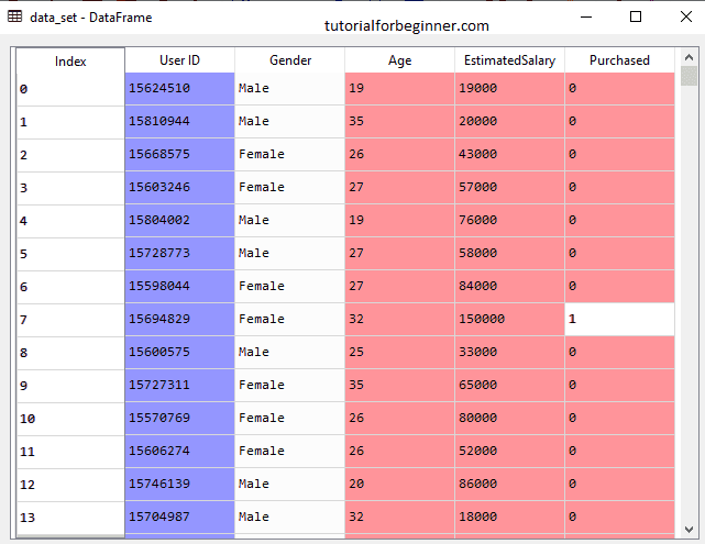
In the above code, we have pre-processed the data. Where we have loaded the dataset, which is given as:
2. Fitting the Random Forest algorithm to the training set:
The Random forest algorithm will now be fitted to the training set. We'll use the RandomForestClassifier class from the sklearn.ensemble package to make it fit. The code is as follows:
   #Fitting Decision Tree classifier to the training set
   from sklearn.ensemble import RandomForestClassifier
   classifier = RandomForestClassifier(n_estimators = 10, criterion = "entropy")
   classifier.fit(x_train, y_train)
The classifier object in the given code has the following parameters:
- n_estimators= The required number of trees in the Random Forest is n estimators. 10 is the default value. We can choose any number, but we must consider the issue of overfitting.
- criterion= This is a function that evaluates the split's correctness. For the information gain, we've used "entropy."
Output:
RandomForestClassifier(bootstrap=True, class_weight=None, criterion='entropy',
  max_depth = None, max_features = 'auto', max_leaf_nodes = None,
  min_impurity_decrease = 0.0, min_impurity_split = None,
  min_samples_leaf = 1, min_samples_split = 2,
  min_weight_fraction_leaf = 0.0, n_estimators = 10,
  n_jobs = None, oob_score = False, random_state = None,
  verbose = 0, warm_start = False)
3. Predicting the Test Set result
We can now anticipate the test outcome because our model has been fitted to the training data. We'll make a new prediction vector, y_pred, for prediction. The code for it is as follows:
   #Predicting the test set result
   y_pred= classifier.predict(x_test)
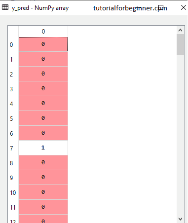
Output:
The prediction vector is given as:
4. Creating the Confusion Matrix
Now we'll make the confusion matrix to figure out which forecasts are true and which are incorrect. The code for it is as follows:
   #Creating the Confusion matrix
   from sklearn.metrics import confusion_matrix
   cm = confusion_matrix(y_test, y_pred)
Output:
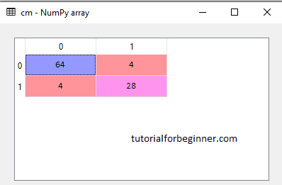
As we can see in the above matrix, there are 4+4= 8 incorrect predictions and 64+28= 92 correct predictions.
5. Visualizing the training Set result
The result of the training set will be visualized here. We will plot a graph for the Random forest classifier to visualize the training set outcome. As we saw in Logistic Regression, the classifier will predict yes or no for consumers who have purchased or not purchased the SUV car. The code for it is as follows:
   from matplotlib.colors import ListedColormap
   x_set, y_set = x_train, y_train
   x1, x2 = nm.meshgrid(nm.arange(start = x_set[:, 0].min() - 1, stop = x_set[:, 0].max() + 1, step  =0.01),
   nm.arange(start = x_set[:, 1].min() - 1, stop = x_set[:, 1].max() + 1, step = 0.01))
   mtp.contourf(x1, x2, classifier.predict(nm.array([x1.ravel(), x2.ravel()]).T).reshape(x1.shape),
   alpha = 0.75, cmap = ListedColormap(('purple','green' )))
   mtp.xlim(x1.min(), x1.max())
   mtp.ylim(x2.min(), x2.max())
   for i, j in enumerate(nm.unique(y_set)):
     mtp.scatter(x_set[y_set == j, 0], x_set[y_set == j, 1],
       c = ListedColormap(('purple', 'green'))(i), label = j)
   mtp.title('Random Forest Algorithm (Training set)')
   mtp.xlabel('Age')
   mtp.ylabel('Estimated Salary')
   mtp.legend()
   mtp.show()
Output:
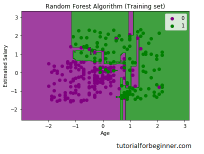
The visualization result for the Random Forest classifier
using the training set result is shown above. It looks a lot
like the Decision tree classifier. The purple and green zones
are the prediction regions, and each data point corresponds to
each user in the user data. Users who did not purchase an SUV
automobile are classed in the purple region, while those who
did purchase an SUV are classified in the green region.
So we took 10 trees in the Random Forest classifier that
predicted Yes or NO for the Purchased variable. The classifier
calculated the result based on the majority of the
predictions.
6. Visualizing the test set result
Now we will visualize the test set result. Below is the code for it:
   #Visulaizing the test set result
   from matplotlib.colors import ListedColormap
   x_set, y_set = x_test, y_test
   x1, x2 = nm.meshgrid(nm.arange(start = x_set[:, 0].min() - 1, stop = x_set[:, 0].max() + 1, step  =0.01),
   nm.arange(start = x_set[:, 1].min() - 1, stop = x_set[:, 1].max() + 1, step = 0.01))
   mtp.contourf(x1, x2, classifier.predict(nm.array([x1.ravel(), x2.ravel()]).T).reshape(x1.shape),
   alpha = 0.75, cmap = ListedColormap(('purple','green' )))
   mtp.xlim(x1.min(), x1.max())
   mtp.ylim(x2.min(), x2.max())
   for i, j in enumerate(nm.unique(y_set)):
     mtp.scatter(x_set[y_set == j, 0], x_set[y_set == j, 1],
       c = ListedColormap(('purple', 'green'))(i), label = j)
   mtp.title('Random Forest Algorithm(Test set)')
   mtp.xlabel('Age')
   mtp.ylabel('Estimated Salary')
   mtp.legend()
   mtp.show()
Output:
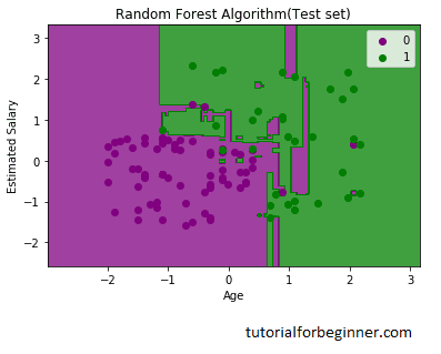
The visualization result for the test set is shown above. Without the Overfitting problem, we can confirm that there are a minimum of (8) inaccurate predictions. Changing the number of trees in the classifier yields varied outcomes.