Apriori Algorithm in Machine Learning
In this page we will learnWhat is Apriori Algorithm in Machine Learning?, What is Frequent Itemset?, Steps for Apriori Algorithm, Apriori Algorithm Working, Advantages of Apriori Algorithm, Disadvantages of Apriori Algorithm, Python Implementation of Apriori Algorithm, Training the Apriori Model on the dataset.
What is Apriori Algorithm in Machine Learning?
The Apriori algorithm generates association rules by using frequent itemsets, and it is designed to work with transaction databases. It determines how strongly or weakly two things are associated using these association rules. To efficiently calculate the itemset relationships, this algorithm use a breadth-first search and a Hash Tree. It is an iterative method for locating common itemsets in a large dataset.
In the year 1994, R. Agrawal and Srikant presented this algorithm. It is mostly used for market basket analysis, which aids in the discovery of products that can be purchased together. It's also useful in the medical field for detecting drug interactions
What is Frequent Itemset?
Itemsets that have a higher level of support than the threshold value or the user-specified minimum level of support are called frequent itemsets. It means that if A and B are frequent itemsets together, then A and B should also be frequent itemsets separately.
Assume there are two transactions: A=1,2,3,4,5, and B=2,3,7; the frequent itemsets in these two transactions are 2 and 3.
[ Note: Understanding association rule learning is recommended to better comprehend the apriori algorithm and related terms such as support and confidence. ]
Steps for Apriori Algorithm
The steps for the apriori algorithm are as follows:
Step 1: Determine the transactional database's support for itemsets and choose the lowest level of support and confidence.
Step 2: Select all supports in the transaction that have a higher support value than the minimum or chosen support value.
Step 3: Identify all of these subsets' rules with a greater confidence value than the threshold or minimal confidence.
Step 4: Arrange the rules in ascending sequence of lift.
Apriori Algorithm Working
Using an example and a mathematical calculation, we will learn about the apriori algorithm:
Assume we have the following dataset with multiple transactions, and we need to locate the frequent itemsets and construct the association rules using the Apriori technique from this dataset:
| TID | ATEMSETS |
|---|---|
| T1 | A, B |
| T2 | B, D |
| T3 | B, C |
| T4 | A, B, D |
| T5 | A, C |
| T6 | B, C |
| T7 | A, C |
| T8 | A, B, C, E |
| T9 | A, B, C |
Solution:
Step-1: Calculating C1 and L1:
- In the first stage, we'll make a table with the support count (the number of times each itemet appears in the dataset) for each itemet in the dataset. The Candidate set, or C1, is the name given to this table.
| Itemset | Support_Count |
|---|---|
| A | 6 |
| B | 7 |
| C | 5 |
| D | 2 |
| E | 1 |
- We'll now remove all the itemets with a higher support count than the Minimum Support (2). It will provide us with the table for the L1 frequently used itemset. With the exception of E, all of the itemsets have larger or equal support counts than the minimal support, hence E will be deleted.
| Itemset | Support_Count |
|---|---|
| A | 6 |
| B | 7 |
| C | 5 |
| D | 2 |
Step-2: Candidate Generation C2, and L2:
- With the help of L1, we will generate C2 in this stage. In C2, we'll make the pair of L1 itemsets in the form of subsets.
- We'll retrieve the support count from the main transaction table of datasets after we've created the subsets, which is how many times these pairs have occurred together in the current dataset. As a result, we'll receive the following table for C2:
| Itemset | Support_Count |
|---|---|
| {A, B} | 4 |
| {A, C} | 4 |
| {A, D} | 1 |
| {B, C} | 4 |
| {B, D} | 2 |
| {C, D} | 0 |
- The C2 Support count must be compared to the minimum support count once more, and the itemset with the lowest support count will be removed from the table C2. It will provide us with the table below for L2.
| Itemset | Support_Count |
|---|---|
| {A, B} | 4 |
| {A, C} | 4 |
| {B, C} | 4 |
| {B, D} | 2 |
A, B, C, D
Step-3: Candidate generation C3, and L3:
- For C3, we'll repeat the first two steps, but this time we'll create the C3 table by combining subsets of three itemsets and calculating the support count from the dataset. It will produce the following table:
| Itemset | Support_Count |
|---|---|
| {A, B, C} | 2 |
| {B, C, D} | 1 |
| {A, C, D} | 0 |
| {A, B, D} | 0 |
- We'll now make the L3 table. As seen in the C3 table above, there is only one itemet combination with
- a support count equal to the minimum support count. As a result, the L3 will only have one combination, namely A, B, and C.
Step-4: Finding the association rules for the subsets:
To construct the association rules, we'll start by creating a new table with all of the potential rules from the A, B.C combination. We'll use the formula sup( A ^B)/A to determine the Confidence for all of the rules. We will exclude the rules that have less confidence than the minimum threshold after calculating the confidence value for all rules (50 % ).
Consider the below table:
| Rules | Support | Confidence |
|---|---|---|
| A ^B → C | 2 | Sup{(A ^B) ^C}/sup(A ^B)= 2/4=0.5=50% |
| B^C → A | 2 | Sup{(B^C) ^A}/sup(B ^C)= 2/4=0.5=50% |
| A^C → B | 2 | Sup{(A ^C) ^B}/sup(A ^C)= 2/4=0.5=50% |
| C→ A ^B | 2 | Sup{(C^( A ^B)}/sup(C)= 2/5=0.4=40% |
| A→ B^C | 2 | Sup{(A^( B ^C)}/sup(A)= 2/6=0.33=33.33% |
| B→ B^C | 2 | Sup{(B^( B ^C)}/sup(B)= 2/7=0.28=28% |
As the given threshold or minimum confidence is 50%, so the first three rules A ^B → C, B^C → A, and A^C → B can be considered as the strong association rules for the given problem.
Advantages of Apriori Algorithm
- This algorithm is simple to comprehend.
- On big datasets, the algorithm's join and prune steps are simple to implement.
Disadvantages of Apriori Algorithm
- In comparison to other algorithms, the apriori algorithm is slow.
- Because it checks the database many times, the overall performance may suffer.
- The apriori algorithm has a time and space complexity of O(2D), which is extremely high. The horizontal width of the database is represented by D.
Python Implementation of Apriori Algorithm
Now we'll look into how the Apriori Algorithm works in practice. To put this into practice, we have a problem with a retailer who wants to find the link between his store's products so that he may offer his consumers a "Buy this, Get that" deal.
The shopkeeper possesses a dataset of information that includes a list of his customer's transactions. Each row in the dataset represents the products that customers have purchased or the transactions that they have performed. We'll take the following actions to remedy this issue:
- Data Pre-processing
- Training the Apriori model on the dataset
- Visualizing the results
1. Data Pre-processing Step:
Data pre-processing is the first step. The first step will be to import the libraries. The following is the code for this:
Importing the libraries: Before we import the libraries, we'll use the following piece of code to install the apyori package, which isn't included in the Spyder IDE:
pip install apyroi
The following is the code for implementing the libraries that will be used for the model's various tasks:
   import numpy as nm
   import matplotlib.pyplot as mtp
   import pandas as pd
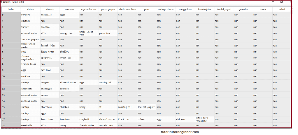
Importing the dataset: The dataset for our apriori model will now be imported. There will be some adjustments here in order to import the dataset. The customers' transactions are represented in all of the rows of the dataset. The first row represents the first customer's transaction, which means that each column has its own name and has its own value or product information (See the dataset given below after the code). As a result, we must state in our code that no header is given. The code is as follows:
   #Importing the dataset
   dataset = pd.read_csv('Market_Basket_data1.csv')
   transactions = []
   for i in range(0, 7501):
     transactions.append([str(dataset.values[i,j])  for j in range(0,20)
The first line of the code above shows how to import the dataset into pandas format. Because the apriori() function that we will use to train our model takes the dataset in the format of a list of transactions, the second line of code is used. As a result, we've constructed an empty transaction list. This list will include all itemsets ranging from 0 to 7500. Because the last index is ignored in Python, we've chosen 7501 here.
The following is an example of the dataset:
2. Training the Apriori Model on the dataset
To train the model, we'll utilize the apriori function from the apyroi package, which will be loaded. The rules for training the model on the dataset will be returned by this function. Consider the code below:
The first line of the preceding code imports the apriori function. The apriori function returns the output as the rules in the second line. It requires the following inputs:
- transactions: The term "transactions" refers to a list of transactions.
- min support= To specify the minimum float value for support. We've used 0.003 here, which is computed by dividing the total number of transactions by three transactions per customer every week.
- min_confidence: Set the minimum confidence value using min confidence. We've taken 0.2 in this case. It can be adjusted depending on the business problem.
- min_lift= To set the minimum lift value.
- min_length= It takes the minimum number of products for the association.
- max_length = It takes the maximum number of products for the association.
3. Visualizing the result
Now we will visualize the output for our apriori model. Here we will follow some more steps, which are given below:
Displaying the result of the rules occurred from the apriori function
   results= list(rules)
   results
By executing the above lines of code, we will get the 9 rules. Consider the below output:
Output:
   [RelationRecord(items=frozenset({'chicken', 'light cream'}), support=0.004533333333333334, ordered_statistics=[OrderedStatistic(items_base=frozenset({'light cream'}), items_add=frozenset({'chicken'}), confidence=0.2905982905982906, lift=4.843304843304844)]),
   RelationRecord(items=frozenset({'escalope', 'mushroom cream sauce'}), support=0.005733333333333333, ordered_statistics=[OrderedStatistic(items_base=frozenset({'mushroom cream sauce'}), items_add=frozenset({'escalope'}), confidence=0.30069930069930073, lift=3.7903273197390845)]),
   RelationRecord(items=frozenset({'escalope', 'pasta'}), support=0.005866666666666667, ordered_statistics=[OrderedStatistic(items_base=frozenset({'pasta'}), items_add=frozenset({'escalope'}), confidence=0.37288135593220345, lift=4.700185158809287)]),
   RelationRecord(items=frozenset({'fromage blanc', 'honey'}), support=0.0033333333333333335, ordered_statistics=[OrderedStatistic(items_base=frozenset({'fromage blanc'}), items_add=frozenset({'honey'}), confidence=0.2450980392156863, lift=5.178127589063795)]),
   RelationRecord(items=frozenset({'ground beef', 'herb & pepper'}), support=0.016, ordered_statistics=[OrderedStatistic(items_base=frozenset({'herb & pepper'}), items_add=frozenset({'ground beef'}), confidence=0.3234501347708895, lift=3.2915549671393096)]),
   RelationRecord(items=frozenset({'tomato sauce', 'ground beef'}), support=0.005333333333333333, ordered_statistics=[OrderedStatistic(items_base=frozenset({'tomato sauce'}), items_add=frozenset({'ground beef'}), confidence=0.37735849056603776, lift=3.840147461662528)]),
   RelationRecord(items=frozenset({'olive oil', 'light cream'}), support=0.0032, ordered_statistics=[OrderedStatistic(items_base=frozenset({'light cream'}), items_add=frozenset({'olive oil'}), confidence=0.20512820512820515, lift=3.120611639881417)]),
   RelationRecord(items=frozenset({'olive oil', 'whole wheat pasta'}), support=0.008, ordered_statistics=[OrderedStatistic(items_base=frozenset({'whole wheat pasta'}), items_add=frozenset({'olive oil'}), confidence=0.2714932126696833, lift=4.130221288078346)]),
   RelationRecord(items=frozenset({'pasta', 'shrimp'}), support=0.005066666666666666, ordered_statistics=[OrderedStatistic(items_base=frozenset({'pasta'}), items_add=frozenset({'shrimp'}), confidence=0.3220338983050848, lift=4.514493901473151)])]
As can be seen, the above output is written in a difficult-to-understand format. As a result, we'll print all of the rules in an appropriate format.
- More clearly visualizing the rule, support, confidence, and lift:
   for item in results:
     pair = item[0]
     items = [x for x in pair]
     print("Rule: " + items[0] + " -> " + items[1])

     print("Support: " + str(item[1]))
     print("Confidence: " + str(item[2][0][2]))
     print("Lift: " + str(item[2][0][3]))
     print("====================================")
By executing the above lines of code, we will get the below output:
   Rule: chicken -> light cream
   Support: 0.004533333333333334
   Confidence: 0.2905982905982906
   Lift: 4.843304843304844
   =====================================
   Rule: escalope -> mushroom cream sauce
   Support: 0.005733333333333333
   Confidence: 0.30069930069930073
   Lift: 3.7903273197390845
   =====================================
   Rule: escalope -> pasta
   Support: 0.005866666666666667
   Confidence: 0.37288135593220345
   Lift: 4.700185158809287
   =====================================
   Rule: fromage blanc -> honey
   Support: 0.0033333333333333335
   Confidence: 0.2450980392156863
   Lift: 5.178127589063795
   =====================================
   Rule: ground beef -> herb & pepper
   Support: 0.016
   Confidence: 0.3234501347708895
   Lift: 3.2915549671393096
   =====================================
   Rule: tomato sauce -> ground beef
   Support: 0.005333333333333333
   Confidence: 0.37735849056603776
   Lift: 3.840147461662528
   =====================================
   Rule: olive oil -> light cream
   Support: 0.0032
   Confidence: 0.20512820512820515
   Lift: 3.120611639881417
   =====================================
   Rule: olive oil -> whole wheat pasta
   Support: 0.008
   Confidence: 0.2714932126696833
   Lift: 4.130221288078346
   =====================================
   Rule: pasta -> shrimp
   Support: 0.005066666666666666
   Confidence: 0.3220338983050848
   Lift: 4.514493901473151
Each rule can be deduced from the above output. The first rule, Light cream chicken, asserts that most customers purchase light cream and chicken on a regular basis. This rule has 0.0045 support and a confidence level of 29 percent. As a result, if a consumer buys light cream, there's a 29 percent probability he'll also buy chicken, and chicken appears.0045 times in the transactions. All of these items can be checked in other rules as well.