Regression Analysis in Machine Learning
Table of Contents:
- Introduction to Regression Analysis
- Enhanced Conceptual Understanding
- Advanced Insights of Regression in Machine Learning
- Applications of Regression Analysis
- Key Terminologies in Regression Analysis
- Importance of Regression Analysis in Machine Learning
- Types of Regression Analysis
- Conclusion
Content Highlight:
This article provides an in-depth exploration of regression analysis, covering its key concepts, types, and applications in machine learning. It includes:
- An introduction to the significance of regression in predictive modeling.
- Detailed explanations of linear, logistic, polynomial, and other advanced regression techniques.
- Real-world examples and scenarios demonstrating the practical applications of regression analysis.
- A conclusion that underscores the importance of regression techniques in modern machine learning.
Introduction to Regression Analysis
Regression analysis is a sophisticated statistical approach used in machine learning to model the relationship between a dependent (target) variable and one or more independent (predictor) variables. Its primary function is to predict continuous outcomes, such as temperature, age, salary, or price, by analyzing how changes in the independent variables affect the target variable, while holding other factors constant. This technique is fundamental in scenarios where understanding and forecasting trends, behaviors, or outcomes is crucial.
Enhanced Conceptual Understanding of Regression Analysis
Regression techniques are not just limited to predictive modeling but are also valuable for interpreting relationships between variables, enabling data scientists and researchers to make informed decisions based on quantified data patterns.
Real-World Scenario: Predicting Sales Based on Advertising
Suppose a marketing company, Company A, allocates a specific budget for advertising every year and tracks its annual sales performance. The table below shows the advertising expenditure over the last five years and the corresponding sales revenue generated:
| Year | Advertising Spend ($) | Sales ($) |
|---|---|---|
| 2015 | 150 | 1200 |
| 2016 | 180 | 1400 |
| 2017 | 200 | 1600 |
| 2018 | 220 | 1750 |
| 2019 | 250 | 1900 |
Now, in 2020, the company plans to allocate $300 for advertising and seeks to predict the expected sales for the year. By applying regression analysis, the relationship between advertising spend and sales can be modeled. Once the model is trained on historical data, the predicted sales for 2020 can be estimated by extending the model to account for the new advertising budget.
This type of forecasting becomes invaluable for companies seeking to make data-driven marketing decisions, optimize their budget allocation, and improve their return on investment (ROI).
Advanced Insights of Regression in Machine Learning
Regression is classified as a supervised learning technique, designed to capture relationships between variables and predict continuous output values. It is widely used not only for forecasting and predictions but also for uncovering causal-effect relationships between variables and for time series modeling. In machine learning, regression models enable automated systems to analyze data and predict outcomes based on historical patterns.
The main task in regression is to fit a function (a regression line or curve) that best represents the relationship between the input (independent) variables and the target (dependent) variable. This is achieved by minimizing the difference (also known as the error or residual) between the observed data points and the predicted values from the model.
In essence, regression aims to produce a line or curve that minimizes the vertical distance between the data points and the regression line. The magnitude of this distance indicates how well the model captures the underlying relationship between the variables. A strong relationship suggests that the model is accurate in explaining the variations in the dependent variable.
Applications of Regression Analysis
Regression analysis is commonly applied in the following fields:
- Weather Forecasting: Predicting temperature or precipitation levels based on atmospheric data such as humidity, wind speed, and air pressure.
- Market Trend Analysis: Forecasting stock market trends, real estate prices, or consumer demand based on historical economic and market data.
- Accident Risk Prediction: Estimating the likelihood of road accidents based on factors such as weather conditions, traffic density, and road quality.
- Medical Prognosis: Predicting patient outcomes based on diagnostic features, medical history, and treatment responses.
Key Terminologies in Regression Analysis
- Dependent Variable (Target): The outcome variable that the regression model aims to predict. In our sales prediction example, the dependent variable is sales.
- Independent Variables (Predictors): The input factors that influence the dependent variable. In the sales prediction example, advertising spend is the independent variable.
- Residuals: The difference between the observed values and the predicted values. The smaller the residuals, the better the model fits the data.
- Multicollinearity: A phenomenon where two or more independent variables are highly correlated, making it difficult to determine the individual impact of each variable on the target. Advanced techniques, such as Variance Inflation Factor (VIF) analysis, are used to detect and mitigate multicollinearity.
- Overfitting: Occurs when the model is excessively complex and captures noise or random fluctuations in the data, resulting in poor generalization to new, unseen data. Regularization techniques, such as Ridge Regression or Lasso Regression, are used to prevent overfitting.
- Underfitting: Happens when the model is too simplistic and fails to capture the true relationships in the data, leading to poor predictive performance.
Importance of Regression Analysis in Machine Learning
As the complexity of data and the need for precise forecasting grows, regression analysis provides invaluable insights. It enables the following:
- Quantification of Relationships: By modeling the relationship between variables, regression helps quantify the impact of changes in predictor variables on the target variable, offering actionable insights.
- Predictive Power: It allows data scientists to predict real-world, continuous outcomes (e.g., pricing, temperature) with a high degree of accuracy, making it an essential tool for decision-makers.
- Causal Inference: Regression helps establish which independent variables are most influential in determining the target variable. This is critical in fields like medicine, economics, and marketing, where understanding cause and effect is paramount.
- Trend Detection: With regression, patterns in historical data can be identified, enabling trend analysis and forward-looking projections, such as predicting consumer behavior or stock market movements.
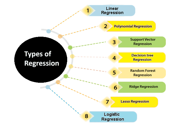
Types of Regression Analysis
In the fields of data science and machine learning, various regression techniques are employed to understand and model the relationships between independent variables (predictors) and dependent variables (targets). Each type of regression serves a distinct purpose, and choosing the right approach is crucial for accurate analysis and predictions. Below, we explore the most important and widely used types of regression:
- Linear Regression
- Logistic Regression
- Polynomial Regression
- Support Vector Regression
- Decision Tree Regression
- Random Forest Regression
- Ridge Regression
- Lasso Regression
Linear Regression: An Overview
Linear regression is a fundamental statistical method utilized in predictive analysis. It is one of the most straightforward yet effective algorithms that demonstrate the relationship between continuous variables. This technique is primarily used for solving regression problems within the field of machine learning.
At its core, linear regression models the linear relationship between an independent variable (X-axis) and a dependent variable (Y-axis), which is why it is aptly named linear regression.
Types of Linear Regression
- Simple Linear Regression: When there is only one independent variable (x), the method is referred to as simple linear regression. It fits a straight line to the data points, representing the relationship between the predictor and the target variable.
- Multiple Linear Regression: When more than one independent variable is involved, the technique is called multiple linear regression. This extends the simple linear regression concept to accommodate more complex relationships by fitting a multidimensional plane through the data points.
The relationship between the variables in a linear regression model can be mathematically expressed as:
Where:
- Y represents the dependent variable (target variable).
- X represents the independent variable(s) (predictor variables).
- a is the slope or coefficient, indicating the rate of change in Y for a unit change in X.
- b is the intercept, representing the value of Y when X is zero.
This equation defines the line that best fits the data, minimizing the difference between observed and predicted values.
Applications of Linear Regression
Linear regression is widely applicable across various fields due to its simplicity and effectiveness. Some popular applications include:
- Analyzing Trends and Sales Estimates: It is used to forecast sales and market trends by analyzing historical data.
- Salary Forecasting: Estimating an employee’s salary based on factors such as years of experience.
- Real Estate Prediction: Predicting property prices based on features like location, size, and amenities.
- Arriving at ETAs in Traffic: Estimating expected time of arrival (ETA) in traffic based on factors like distance, speed, and road conditions.
Linear regression remains a cornerstone in statistical modeling, providing clear and actionable insights across numerous practical scenarios.
The image below is a classic example of how Linear Regression can be applied to understand and predict the relationship between an employee's experience (measured in years) and their salary. This type of regression is widely used in predictive analysis within machine learning and data science.
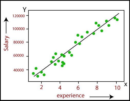
In this graph:
- X-axis represents the number of years of experience an employee has.
- Y-axis represents the salary of the employee.
- The green dots are the actual data points that show observed salaries corresponding to various levels of experience.
- The black line is the regression line, which is the best-fit line calculated by the linear regression model to represent the relationship between experience and salary.
This graph visually demonstrates that as the employee’s experience increases, their salary also tends to increase. The upward slope of the regression line indicates a positive relationship between these two variables. The purpose of this line is to predict the salary based on years of experience. The model aims to minimize the difference between the predicted salaries (represented by the line) and the actual observed salaries (represented by the green dots).
This visualization helps in understanding the practical applications of linear regression for making informed predictions and analyzing trends within datasets.
Logistic Regression
Logistic regression is a widely-used supervised learning algorithm specifically designed to tackle classification problems. Unlike other regression models, logistic regression is ideal for scenarios where the dependent variable is in a binary or discrete format, such as 0 or 1.
This algorithm works effectively with categorical variables, where the possible outcomes are distinct categories like Yes or No, True or False, or Spam or Not Spam. Logistic regression is fundamentally a predictive analysis technique that operates on the principles of probability.
Although logistic regression is classified as a type of regression, it differs significantly from linear regression in how it is applied. Specifically, logistic regression employs the sigmoid function (also known as the logistic function), which is a complex cost function used to model the data.
The Sigmoid Function in Logistic Regression
The sigmoid function transforms the input values into an output that falls between 0 and 1. Mathematically, it can be represented as:
1 + e-x
Where:
- f(x) is the output value between 0 and 1.
- x is the input to the function.
- e is the base of the natural logarithm.
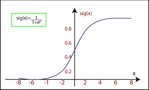
When the input values (data) are fed into this function, it generates an S-shaped curve, which is why it's often referred to as the S-curve.
This S-curve allows logistic regression to handle classification by applying a threshold level. Any values above the threshold are classified as 1, and those below are classified as 0.
Polynomial Regression: Modeling Non-Linear Relationships
Polynomial Regression is another powerful regression technique designed to model datasets that exhibit a non-linear relationship. While it shares similarities with multiple linear regression, it introduces non-linearity by fitting a polynomial curve to the data.
When a dataset contains data points that are distributed in a non-linear fashion, linear regression might not be the best fit. This is where polynomial regression becomes essential. It transforms the original features into polynomial features of a given degree and models them using a linear approach.
Polynomial Regression Equation:
The equation for polynomial regression is derived from the linear regression equation but is expanded to include higher-degree terms:
Where:
- Y is the predicted (target) output.
- X represents the independent (input) variable.
- b0, b1, ...... , bn are the regression coefficients for each degree of the polynomial.
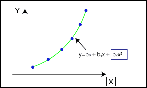
While the model remains linear in terms of the coefficients, the inclusion of quadratic, cubic, and higher-degree terms allows it to capture non-linear patterns in the data effectively.
Support Vector Regression
Support Vector Machine (SVM) is a versatile supervised learning algorithm that can be applied to both classification and regression problems. When this algorithm is used for regression tasks, it is specifically referred to as Support Vector Regression (SVR).
Support Vector Regression (SVR) is a robust regression algorithm designed to work effectively with continuous variables. It aims to predict outcomes within a certain range by determining a hyperplane that best fits the data points within a specified margin.
Key Concepts in Support Vector Regression (SVR)
- Kernel: A function used to map lower-dimensional data into a higher-dimensional space, enabling the algorithm to handle non-linear relationships more effectively.
- Hyperplane: In the context of SVM, the hyperplane is a line that separates different classes in classification tasks. In SVR, however, it serves as the best-fit line that predicts continuous variables while covering most of the data points within the defined margin.
- Boundary Lines: These are the two lines drawn parallel to the hyperplane. They create a margin within which the data points are allowed to fall. The goal is to maximize the margin between these boundary lines.
- Support Vectors: The data points that are closest to the hyperplane and lie within the margin. These support vectors are critical in defining the position and orientation of the hyperplane.
The primary objective of SVR is to determine a hyperplane with a maximum margin so that the maximum number of data points fall within this margin. This ensures that the model generalizes well and can make accurate predictions.

In the image above:
- The blue line represents the hyperplane, which is the best-fit line determined by the SVR model.
- The two dashed lines are the boundary lines, marking the margins within which the data points are expected to fall.
- The green dots are the data points, most of which fall within the margin, demonstrating the model's effectiveness in capturing the relationship between the variables.
This approach makes Support Vector Regression a powerful tool in the realm of machine learning, especially when dealing with data that exhibits continuous trends.
Decision Tree Regression
Decision Tree Regression is a powerful supervised learning algorithm that can be used to solve both classification and regression problems. This versatile algorithm is capable of handling both categorical and numerical data, making it a go-to choice for many machine learning tasks.
In Decision Tree Regression, a tree-like structure is built where each internal node represents a "test" for an attribute, each branch represents the outcome of the test, and each leaf node represents the final decision or result. The tree starts with a root node (the entire dataset) and splits into child nodes based on the attributes that best separate the data. These child nodes are further divided, continuing the process until the tree reaches its leaf nodes.
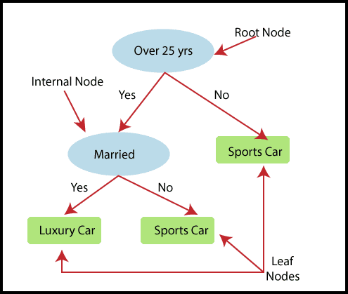
In the above image, the Decision Tree Regression model is predicting a person’s choice between a Sports Car and a Luxury Car. The tree starts with the root node that tests whether the person is over 25 years old. Depending on the answer, it moves through the nodes, testing marital status, and ultimately predicting the preferred car type.
Random Forest Regression
Random Forest Regression is an advanced ensemble learning technique that builds upon the strengths of multiple decision trees. It is one of the most robust and accurate supervised learning algorithms, capable of performing both classification and regression tasks.
In Random Forest Regression, multiple decision trees are constructed and combined to predict the final output. Each tree in the forest makes its own prediction, and the final prediction is derived by averaging all the individual tree predictions. This method, known as Bagging or Bootstrap Aggregation, helps to reduce the risk of overfitting and improves the model’s accuracy.
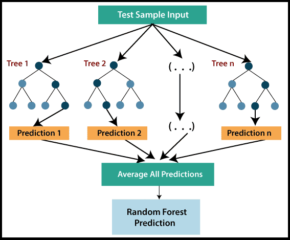
As depicted in the image above, the Random Forest Regression model begins with a test sample input, which is passed through multiple trees (Tree 1, Tree 2, …, Tree n). Each tree makes a prediction, and these predictions are averaged to produce the final output, effectively capturing the nuances of the data.
By leveraging the combined power of multiple decision trees, Random Forest Regression ensures more accurate and reliable predictions, making it a highly preferred choice for complex machine learning tasks.
Ridge Regression
Ridge Regression is one of the most robust variations of linear regression. It introduces a small amount of bias to the model, which helps to achieve more accurate and stable long-term predictions. This bias is known as the Ridge Regression penalty.
The penalty term in Ridge Regression is computed by multiplying a parameter, lambda (λ), by the squared weight of each individual feature. The primary goal of this technique is to prevent overfitting, especially when there is high collinearity among the independent variables.
Ridge Regression Equation
In this equation:
- L(x, y) represents the loss function.
- λ (lambda) controls the strength of the regularization.
- wi are the weights for each feature.
Ridge Regression, also known as L2 regularization, is particularly effective in scenarios where there are more parameters than samples. By reducing the complexity of the model, it helps to ensure more reliable and interpretable predictions.
Lasso Regression
Lasso Regression is another powerful regularization technique used to reduce model complexity. While it shares similarities with Ridge Regression, the key difference lies in the penalty term. In Lasso Regression, the penalty involves the absolute values of the weights rather than their squares.
This unique feature allows Lasso Regression to effectively shrink some coefficients to zero, thereby performing feature selection. This makes Lasso particularly useful when dealing with high-dimensional datasets where many features may be irrelevant.
Lasso Regression Equation
In this equation:
- L(x, y) represents the loss function.
- λ (lambda) controls the strength of the regularization.
- wi are the weights for each feature, and the absolute values ensure some coefficients can be reduced to zero.
Lasso Regression, also known as L1 regularization, is an ideal choice for scenarios where feature selection is crucial. By focusing only on the most important features, it simplifies the model while maintaining accuracy.
Conclusion
Regression analysis stands as a cornerstone of machine learning, offering a range of techniques to model and predict continuous outcomes. From the simplicity of linear regression to the complexity of Ridge and Lasso, each method has its unique advantages and use cases. By understanding and applying these techniques, data scientists can derive valuable insights, make accurate predictions, and drive data-driven decisions across various industries. As machine learning continues to evolve, the importance of mastering regression techniques will only grow, making them indispensable tools in the arsenal of any data scientist.