Linear Regression in ML
Table of Contents:
- What is Linear Regression in Machine Learning?
- Types of Linear Regression
- Understanding the Linear Regression Line
- Finding the Best Fit Line
- Cost Function in Linear Regression
- Gradient Descent in Linear Regression
- Model Performance in Linear Regression
- Assumptions of Linear Regression
- Conclusion
Content Highlight:
Linear regression is a cornerstone of machine learning, renowned for its simplicity and effectiveness in predictive analysis. It models the linear relationship between a dependent variable and one or more independent variables, aiming to find the best-fitting line through data points. This relationship is quantified using coefficients, optimized through the cost function, typically the Mean Squared Error (MSE). Linear regression comes in two forms—Simple and Multiple—depending on the number of predictors, and its performance is evaluated by the R-squared method, which measures the goodness of fit. To ensure the model's reliability, key assumptions such as linearity, minimal multicollinearity, homoscedasticity, normal distribution of error terms, and no autocorrelation must be met.
What is Linear Regression in Machine Learning?
Linear regression is a foundational and widely embraced algorithm in the realm of machine learning. As one of the simplest forms of predictive analysis, it excels in forecasting continuous, real-valued outcomes such as sales figures, salaries, age, product prices, and more. This technique derives its power from its ability to establish and quantify relationships between variables.
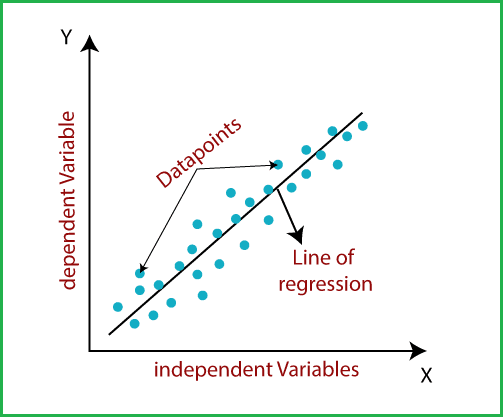
In essence, linear regression uncovers the linear relationship between a dependent variable (often denoted as ( y )) and one or more independent variables (denoted as ( x )). This linearity implies that as the value of the independent variable(s) changes, the dependent variable's value shifts correspondingly. The algorithm attempts to find the best-fitting straight line through the data points, symbolizing this relationship.
Imagine this line as a guide, mapping how changes in the independent variable(s) influence the dependent variable. The sloped nature of this line indicates the direction and magnitude of these changes, offering a clear and interpretable model of prediction.
Visualizing the relationship as a sloped line, the model not only provides insight but also paves the way for making informed predictions, where the dependent variable’s value can be estimated based on the known values of the independent variables.
Mathematical Representation of Linear Regression:
Linear regression can be mathematically expressed as:
y = a0 + a1x + ε
Where:
- y: Dependent Variable (Target Variable)
- x: Independent Variable (Predictor Variable)
- a0: Intercept of the line (Provides an additional degree of freedom)
- a1: Linear regression coefficient (Scale factor applied to each input value)
- ε: Random error term
In this equation, the values for x and y are derived from training datasets used to construct the Linear Regression model.
Types of Linear Regression
Linear regression is categorized into two distinct types based on the number of independent variables:
1. Simple Linear Regression:
This type of linear regression involves a single independent variable used to predict the value of a numerical dependent variable. When the model relies on just one predictor, it is referred to as Simple Linear Regression.
2. Multiple Linear Regression:
In contrast, Multiple Linear Regression involves more than one independent variable to predict the value of a numerical dependent variable. When multiple predictors are considered in the model, it is known as Multiple Linear Regression.
Understanding the Linear Regression Line:
A regression line is a straight line that illustrates the relationship between the dependent and independent variables in linear regression. This line can reveal two types of relationships between the variables: positive and negative linear relationships.
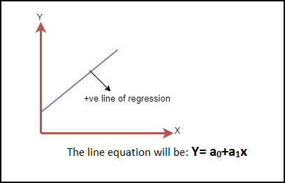
Positive Linear Relationship:
A positive linear relationship occurs when the dependent variable increases along the Y-axis as the independent variable increases along the X-axis. In this scenario, the regression line slopes upwards from left to right, indicating that as one variable increases, so does the other. The equation for a positive regression line is given by:
Y = a0 + a1X
This positive slope signifies that the variables move in the same direction. The image below visually represents a positive linear relationship:
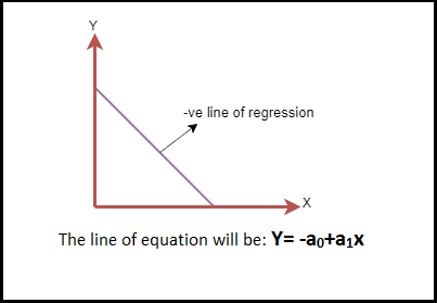
Negative Linear Relationship:
Conversely, a negative linear relationship is characterized by a decrease in the dependent variable along the Y-axis as the independent variable increases along the X-axis. In this case, the regression line slopes downwards from left to right, reflecting an inverse relationship where an increase in one variable leads to a decrease in the other. The equation for a negative regression line is:
Y = -a0 + a1X
This negative slope indicates that the variables move in opposite directions. The image below visually depicts a negative linear relationship:
Finding the Best Fit Line:
In the context of linear regression, the primary objective is to identify the best fit line—a line that minimizes the difference between the predicted values and the actual values. This line should have the least amount of error, making it the most accurate representation of the data.
The accuracy of this fit is determined by the weights or coefficients of the line, represented by a0 (the intercept) and a1 (the slope). Each combination of these values results in a different regression line. The challenge lies in calculating the optimal values for a0 and a1 to ensure that the chosen line best fits the data.
To achieve this, we employ a method known as the cost function. The cost function quantifies the error between the predicted values (derived from the regression line) and the actual values in the dataset. The goal is to minimize this cost function, thereby determining the best possible line for the given data.
By continuously adjusting a0 and a1 and minimizing the cost function, we can derive the optimal regression line that best represents the relationship between the dependent and independent variables in the dataset.
Cost Function in Linear Regression
In linear regression, the cost function is a crucial tool used to estimate the optimal values of the coefficients a0 and a1 that define the regression line. Each combination of these coefficients produces a different regression line, and the cost function helps us find the one that best fits the data.
The primary role of the cost function is to optimize the regression coefficients or weights. It measures how well a linear regression model is performing by evaluating the accuracy of the mapping function, which translates the input variables into the output variables. This mapping function is also referred to as the hypothesis function.
For linear regression, the Mean Squared Error (MSE) is commonly used as the cost function. The MSE is the average of the squared differences between the predicted values and the actual values. Mathematically, it can be represented as:
MSE = 1⁄N Σni=1 (Yi - (a1xi + a0))2
Where:
- N = Total number of observations
- Yi = Actual value
- (a1xi + a0) = Predicted value
The difference between the actual value and the predicted value is known as the residual. If the data points are far from the regression line, the residual will be large, resulting in a higher cost function value. Conversely, if the points are close to the regression line, the residual will be small, leading to a lower cost function value.
Gradient Descent in Linear Regression:
Gradient descent is an optimization technique used to minimize the MSE by calculating the gradient of the cost function. The linear regression model uses gradient descent to iteratively update the coefficients of the line, reducing the cost function in the process.
This is achieved by initially selecting random values for the coefficients and then iteratively adjusting them to find the minimum value of the cost function. By continuously updating the coefficients in the direction that decreases the cost function, the model converges towards the best fit line that accurately represents the data.
In summary, the cost function and gradient descent are essential components of linear regression that work together to optimize the model, ensuring it provides the most accurate predictions possible.
Model Performance in Linear Regression:
Model Performance in linear regression is evaluated by determining how well the regression line fits the observed data points. This is commonly referred to as the Goodness of Fit. The process of selecting the best model from various alternatives is known as optimization. One of the key methods to assess model performance is the R-squared method.
1. R-squared Method
R-squared is a statistical measure that indicates the Goodness of Fit of a regression model. It quantifies the strength of the relationship between the dependent and independent variables on a scale ranging from 0% to 100%. A higher R-squared value indicates a stronger relationship, signifying that the model has a smaller difference between the predicted and actual values, thus representing a better fit.
R-squared is also known as the coefficient of determination or, in the case of multiple regression, the coefficient of multiple determination. It can be calculated using the following formula:
R-squared = Explained variation⁄Total Variation
In this formula:
- Explained variation refers to the portion of the total variation in the dependent variable that the model can explain.
- Total Variation is the overall variation in the dependent variable.
A higher R-squared value implies a better fit of the regression line to the observed data, indicating that the model is well-suited for making accurate predictions.
Assumptions of Linear Regression:
When building a linear regression model, certain assumptions must be met to ensure the accuracy and reliability of the results. These assumptions are critical checks that help in deriving the best possible outcomes from the given dataset. Here are the key assumptions of linear regression:
1. Linear Relationship Between Features and Target
Linear regression assumes a linear relationship between the dependent (target) variable and the independent (feature) variables. This means that changes in the independent variables should proportionally affect the dependent variable.
2. Small or No Multicollinearity Between Features
Multicollinearity refers to a situation where independent variables are highly correlated with each other. High multicollinearity can make it difficult to ascertain the true relationship between the predictors and the target variable. It complicates the determination of which predictor is influencing the target variable. Therefore, the model assumes either little or no multicollinearity among the independent variables to maintain clarity in the relationships.
3. Homoscedasticity Assumption
Homoscedasticity occurs when the error terms (residuals) have constant variance across all levels of the independent variables. In other words, the spread of the residuals should be consistent for all values of the independent variables. When homoscedasticity is present, there should be no discernible pattern in the scatter plot of the residuals, ensuring that the model’s predictions are unbiased.
4. Normal Distribution of Error Terms
Linear regression also assumes that the error terms (differences between observed and predicted values) are normally distributed. If the error terms deviate from a normal distribution, the confidence intervals of the model may become inaccurate—either too wide or too narrow—leading to potential errors in the interpretation of the coefficients. This assumption can be visually checked using a Q-Q plot; if the plot forms a straight line with minimal deviation, the error terms are likely normally distributed.
5. No Autocorrelation of Error Terms
The model assumes that there is no autocorrelation in the error terms. Autocorrelation occurs when residuals (errors) are not independent of each other, which can severely reduce the model’s accuracy. Autocorrelation is particularly problematic in time series data, where residuals might be correlated due to temporal dependencies.
Conclusion:
Linear regression is a fundamental tool in machine learning for predictive analysis, providing a clear and interpretable model for understanding relationships between variables. Its effectiveness hinges on the correct application of assumptions and optimization techniques like the cost function and gradient descent. By adhering to these principles, linear regression models can deliver highly accurate and reliable predictions, making them invaluable in various applications, from forecasting sales to determining product prices and beyond.