Decision Tree Classification Algorithm in Machine Learning
In this page, we will learn Decision Tree Classification Algorithm in Machine Learning, What is Decision Tree Classification Algorithm?, Why use Decision Trees?, Decision Tree Terminologies, How does the Decision Tree algorithm Work?, Attribute Selection Measures, Advantages of the Decision Tree, Disadvantages of the Decision Tree, Python Implementation of Decision Tree.
What is Decision Tree Classification Algorithm?
- Decision Tree is a supervised learning technique that may be used to solve both classification and regression problems, however it is most commonly employed to solve classification issues. Internal nodes represent dataset attributes, branches represent decision rules, and each leaf node provides the conclusion in this tree-structured classifier.
- The Decision Node and the Leaf Node are the two nodes of a Decision tree. Decision nodes are used to make any decision and have several branches, whereas Leaf nodes are the results of such decisions and have no additional branches.
- The decisions or tests are made based on the characteristics of the given dataset.
- It's a graphical depiction for obtaining all feasible solutions to a problem/decision depending on certain parameters.
- It's termed a decision tree because, like a tree, it starts with the root node and grows into a tree-like structure with additional branches.
- We utilize the CART algorithm, which stands for Classification and Regression Tree algorithm, to form a tree.
- A decision tree simply asks a question and divides the tree into subtrees based on the answer (Yes/No).
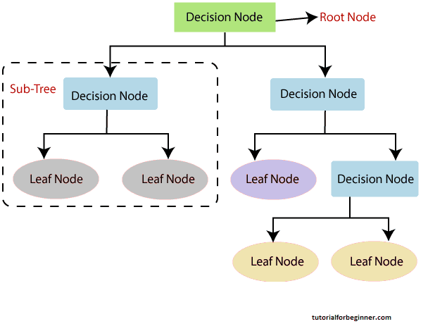
- A decision tree's general structure is seen in the diagram below:
[Note: A decision tree can contain categorical data (YES/NO) as well as numeric data. ]
Why use Decision Trees?
Machine learning uses a variety of algorithms, therefore
picking the optimal approach for the given dataset and problem
is the most important thing to remember while building a
machine learning model. The following are two reasons to use
the Decision Tree:
Decision Trees are designed to mirror human thinking abilities
when making decisions, making them simple to comprehend.
Because the decision tree has a tree-like form, the rationale
behind it is simple to comprehend.
Decision Tree Terminologies
The root node: It is the starting point for the
decision tree. It represents the full dataset, which is then
split into two or more homogeneous groups.
Leaf Node: Leaf nodes are the tree's final output
nodes, and they can't be separated any further after that.
Splitting: Splitting is the process of separating the
decision node/root node into sub-nodes based on the conditions
specified.
Branch/Sub Tree: A tree that has been split into
branches or subtrees.
Pruning: It is the procedure of pruning a tree to
remove undesired branches.
Parent/Child node: The root node of the tree is known
as the parent node, while the remaining nodes are known as the
child nodes.
How does the Decision Tree algorithm Work?
The procedure for determining the class of a given dataset in
a decision tree starts at the root node of the tree. This
algorithm checks the values of the root attribute with the
values of the record (actual dataset) attribute and then
follows the branch and jumps to the next node based on the
comparison.
The algorithm compares the attribute value with the other
sub-nodes and moves on to the next node. It repeats the
process until it reaches the tree's leaf node. The following
algorithm can help you understand the entire process:
Step 1: Start with the root node, which holds the
entire dataset, explains S.
Step 2: Using the Attribute Selection Measure, find the
best attribute in the dataset (ASM).
Step 3: Subdivide the S into subsets that contain the
best attribute's possible values.
Step 4: Create the node of the decision tree that has
the best attribute.
Step 5: Create additional decision trees in a recursive
manner using the subsets of the dataset obtained in step 3.
Continue this process until the nodes can no longer be
classified, at which point the final node is referred to as a
leaf node.
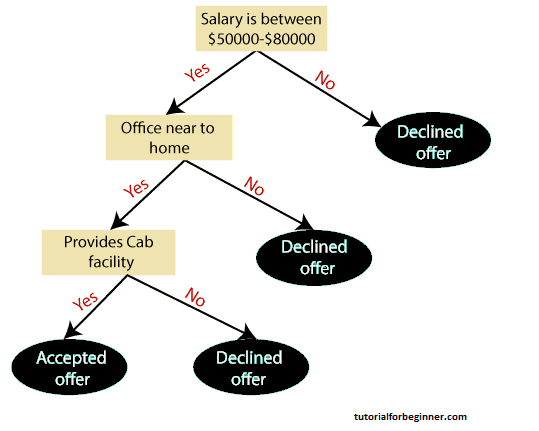
Example: An applicant receives a job offer and must decide whether or not to take it. As a result, the decision tree begins at the root node to answer this problem (Salary attribute by ASM). Based on the corresponding labels, the root node splits into the next decision node (distance from the office) and one leaf node. The following decision node is divided into one decision node (Cab facility) and one leaf node. The decision node eventually splits into two leaf nodes (Accepted offers and Declined offer). Consider the diagram below:
Attribute Selection Measures
The biggest challenge that emerges while developing a Decision tree is how to choose the best attribute for the root node and sub-nodes. So, there is a technique called Attribute Selection Measure, or ASM, that can be used to overcome such situations. We can easily determine the best property for the tree's nodes using this measurement. The following are two popular ASM techniques:
- Information Gain
- Gini Index
Information Gain:
- The assessment of changes in entropy after segmenting a dataset based on an attribute is known as information gain.
- It determines how much data a feature offers about a class.
- We split the node and built the decision tree based on the value of information gained.
-
The highest information gain node/attribute is split first
in a decision tree method, which always strives to maximize
the value of information gain. The following formula can be
used to compute it:
Information Gain= Entropy(S)- [(Weighted Avg) *Entropy(each feature)
Entropy: It is a metric for determining the degree of
impurity in a particular property. It denotes the randomness
of data. The following formula can be used to compute entropy:
Entropy(s)= -P(yes)log2 P(yes)- P(no) log2 P(no)
Where,
S= Total number of samples
P(yes)= probability of yes
P(no)= probability of no
2. Gini Index:
- The Gini index is a measure of impurity or purity used in the CART (Classification and Regression Tree) technique to create a decision tree.
- In comparison to a high Gini index, an attribute with a low Gini index should be favoured.
- It only makes binary splits, and the CART method creates binary splits using the Gini index.
-
The following formula can be used to compute the Gini index:
Gini Index= 1- ∑ j P j 2
Pruning: Getting an Optimal Decision tree
Pruning is a process of deleting the unnecessary nodes from a
tree in order to get the optimal decision tree.
Overfitting is more likely with a large tree, yet a small tree
may not capture all of the key properties of the dataset.
Pruning is a strategy for reducing the size of the learning
tree without reducing accuracy. Tree pruning technology is
mostly divided into two categories:
- Cost Complexity Pruning
- Reduced Error Pruning.
Advantages of the Decision Tree
- It is straightforward to comprehend because it follows the identical steps that a human would use while making a decision in the actual world.
- It can be extremely helpful in resolving decision-making issues.
- It is beneficial to consider all of the possible solutions to an issue.
- In comparison to other algorithms, data cleansing is not required as much
Disadvantages of the Decision Tree
- The decision tree is complicated since it has several tiers.
- It may have an overfitting problem, which the Random Forest algorithm can solve.
- The computational complexity of the decision tree may increase as additional class labels are added.
Python Implementation of Decision Tree
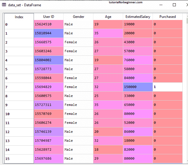
Now we'll use Python to implement the Decision Tree. We'll use
the "user_data.csv" dataset, which we've used in earlier
classification models. We may compare the Decision tree
classifier to other classification models such as KNN SVM,
LogisticRegression, and others using the same dataset.
The steps, which are listed below, will also remain the same.
- Data Pre-processing step
- Fitting a Decision-Tree algorithm to the Training set
- Predicting the test result
- Test accuracy of the result(Creation of Confusion matrix)
- Visualizing the test set result.
1. Data Pre-Processing Step:
Below is the code for the pre-processing step
   #importing libraries
   import numpy as nm
   import matplotlib.pyplot as mtp
   import pandas as pd

   #importing datasets
   data_set = pd.read_csv('user_data.csv')

   #Extracting Independent and dependent Variable
   x = data_set.iloc[:, [2,3]].values
   y = data_set.iloc[:, 4].values

   #Splitting the dataset into training and test set.
   from sklearn.model_selection import train_test_split
   x_train, x_test, y_train, y_test= train_test_split(x, y, test_size = 0.25, random_state = 0)

   #feature Scaling
   from sklearn.preprocessing import StandardScaler
   st_x = StandardScaler()
   x_train = st_x.fit_transform(x_train)
   x_test = st_x.transform(x_test)
In the above code, we have pre-processed the data. Where we have loaded the dataset, which is given as:
2. Fitting a Decision-Tree algorithm to the Training set
We'll now match the model to the training set. We'll use the DecisionTreeClassifier class from the sklearn.tree package for this. The code for it is as follows:
   #Fitting Decision Tree classifier to the training set
   From sklearn.tree import DecisionTreeClassifier
   classifier= DecisionTreeClassifier(criterion = 'entropy', random_state = 0)
   classifier.fit(x_train, y_train)
We constructed a classifier object in the preceding code and passed two major arguments to it;
- "criterion='entropy': Criterion is used to assess the quality of a split, which is determined by entropy's information gain.
- random state=0": For the purpose of producing random states.
The result is as follows:
   DecisionTreeClassifier(class_weight = None, criterion = 'entropy', max_depth = None,
           max_features = None, max_leaf_nodes = None,
           min_impurity_decrease = 0.0, min_impurity_split = None,
           min_samples_leaf = 1, min_samples_split = 2,
           min_weight_fraction_leaf = 0.0, presort = False,
           random_state = 0, splitter = 'best')
Predicting the test result
Now we'll forecast the outcome of the test set. We're going to make a new prediction vector called y pred. The code for it is as follows:
   #Predicting the test set result
   y_pred = classifier.predict(x_test)
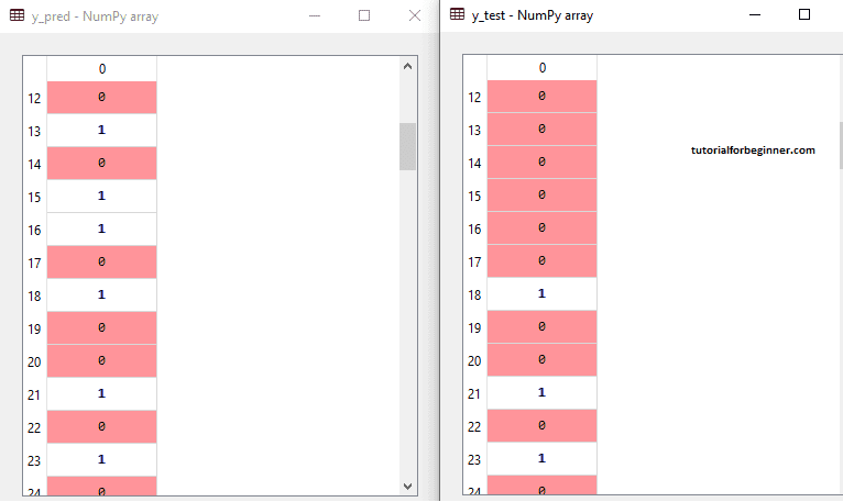
Output:
The expected and real test outputs are shown in the output image below. There are some values in the prediction vector that deviate from the true vector values, as can be seen. These are errors in prediction.
4. Test accuracy of the result (Creation of Confusion matrix)
We can see that there were some wrong guesses in the above output, therefore we'll need to utilize the confusion matrix to figure out how many correct and incorrect predictions there were. The code for it is as follows:
   #Creating the Confusion matrix
   from sklearn.metrics import confusion_matrix
   cm = confusion_matrix(y_test, y_pred)
Output:
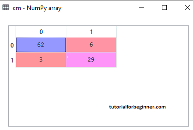
The confusion matrix may be seen in the above output graphic, with 6+3= 9 wrong predictions and 62+29=91 right predictions. As a result, we may conclude that the Decision Tree classifier made an excellent prediction when compared to other classification models.
5. Visualizing the training set result:
The result of the training set will be visualized here. We will plot a graph for the decision tree classifier to visualize the training set outcome. As we saw in Logistic Regression, the classifier will predict yes or no for consumers who have purchased or not purchased the SUV car. The code for it is as follows:
   #Visulaizing the trianing set result
   from matplotlib.colors import ListedColormap
   x_set, y_set = x_train, y_train
   x1, x2 = nm.meshgrid(nm.arange(start = x_set[:, 0].min() - 1, stop = x_set[:, 0].max() + 1, step  =0.01),
   nm.arange(start = x_set[:, 1].min() - 1, stop = x_set[:, 1].max() + 1, step = 0.01))
   mtp.contourf(x1, x2, classifier.predict(nm.array([x1.ravel(), x2.ravel()]).T).reshape(x1.shape),
   alpha = 0.75, cmap = ListedColormap(('purple','green' )))
   mtp.xlim(x1.min(), x1.max())
   mtp.ylim(x2.min(), x2.max())
   fori, j in enumerate(nm.unique(y_set)):
     mtp.scatter(x_set[y_set == j, 0], x_set[y_set == j, 1],
       c = ListedColormap(('purple', 'green'))(i), label = j)
   mtp.title('Decision Tree Algorithm (Training set)')
   mtp.xlabel('Age')
   mtp.ylabel('Estimated Salary')
   mtp.legend()
Output:
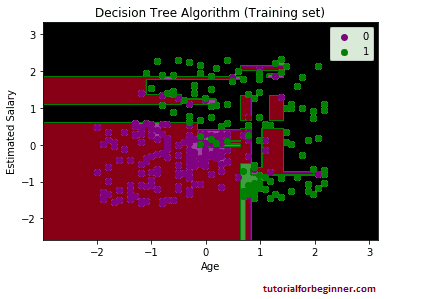
The output seen above differs significantly from the rest of
the classification models. It features both vertical and
horizontal lines that divide the dataset into age and
predicted pay categories.
As can be seen, the tree is attempting to capture each
dataset, resulting in overfitting.
6. Visualizing the test set result:
The test set result will be visualized similarly to the training set result, with the exception that the training set will be substituted with the test set.
   #Visulaizing the test set result
   from matplotlib.colors import ListedColormap
   x_set, y_set = x_test, y_test
   x1, x2 = nm.meshgrid(nm.arange(start = x_set[:, 0].min() - 1, stop = x_set[:, 0].max() + 1, step  =0.01),
   nm.arange(start = x_set[:, 1].min() - 1, stop = x_set[:, 1].max() + 1, step = 0.01))
   mtp.contourf(x1, x2, classifier.predict(nm.array([x1.ravel(), x2.ravel()]).T).reshape(x1.shape),
   alpha = 0.75, cmap = ListedColormap(('purple','green' )))
   mtp.xlim(x1.min(), x1.max())
   mtp.ylim(x2.min(), x2.max())
   for i, j in enumerate(nm.unique(y_set)):
     mtp.scatter(x_set[y_set == j, 0], x_set[y_set == j, 1],
        c = ListedColormap(('purple', 'green'))(i), label = j)
   mtp.title('Decision Tree Algorithm(Test set)')
   mtp.xlabel('Age')
   mtp.ylabel('Estimated Salary')
   mtp.legend()
   mtp.show()
Output:
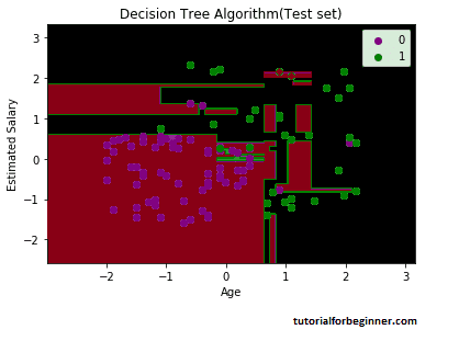
As can be seen in the accompanying graphic, some green data points are contained within the purple zone, and vice versa. So, these are the wrong predictions that we talked about in the confusion matrix.