ML Polynomial Regression in ML
Table of Contents:
- What is Polynomial Regression?
- Why Use Polynomial Regression?
- Equation Comparison
- Implementation of Polynomial Regression using Python
- Steps for Polynomial Regression
- Visualizing Linear vs. Polynomial Regression
- Predicting Results
- Conclusion
Content Highlight:
This guide on Polynomial Regression explains how to model non-linear relationships in Machine Learning. Learn the importance of using a Polynomial Regression model over a linear model when data is non-linear, and follow a detailed step-by-step Python implementation using scikit-learn.
What is Polynomial Regression?
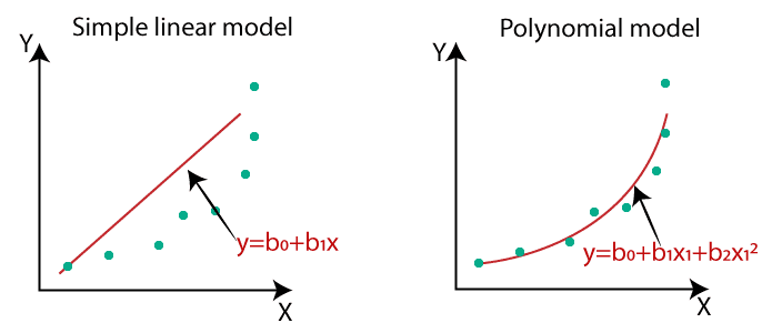
Polynomial Regression is a form of regression analysis that models the relationship between a dependent variable (y) and one or more independent variables (x) as an n-th degree polynomial. Unlike Simple Linear Regression, it can capture non-linear relationships in the data. The regression equation takes the following form:
y = b0 + b1x + b2x2 + ... + bnxn
This makes Polynomial Regression ideal for data with curved patterns that cannot be effectively modeled with a straight line.
Why Use Polynomial Regression?
Polynomial Regression is necessary when the data points are arranged in a non-linear fashion. Applying a linear model to such data often results in high error rates and inaccurate predictions. In contrast, Polynomial Regression provides a curved model that better fits the data, minimizing loss function and enhancing accuracy. It is particularly useful for scenarios like price prediction and weather forecasting, where relationships between variables are complex.
Equation Comparison:
Let’s compare the equations of different regression models to understand the concept:
- Simple Linear Regression: y = b0 + b1x
- Multiple Linear Regression: y = b0 + b1x + b2x2 + ... + bnxn
- Polynomial Regression: y = b0 + b1x + b2x2 + ... + bnxn
All three equations are polynomial in nature but differ by the degree of the variables. Polynomial Regression extends the linear model to higher degrees, making it ideal for capturing complex patterns in the data.
Implementation of Polynomial Regression Using Python
Here, we will implement Polynomial Regression using Python and compare it with Linear Regression. This example uses a Salary Prediction Dataset to predict the salary for a candidate based on position levels.
Problem Description:
A Human Resource (HR) company is in the process of hiring a new candidate. The candidate claims that their previous annual salary was 160K. To verify this claim, the HR team needs to determine if the candidate is being truthful or exaggerating. However, they only have access to a dataset from the candidate’s previous company, which details the salaries associated with the top 10 job positions, along with their respective levels. Upon analyzing this dataset, it becomes evident that there is a non-linear relationship between the job position levels and their corresponding salaries. The objective is to build a regression model capable of detecting any discrepancies in the candidate’s claim. This "Bluff Detection" model will help the HR team make an informed hiring decision, ensuring they bring on board a candidate who is honest about their past compensation.
| Position | Level (X-variable) | Salary (Y-variable) |
|---|---|---|
| Business Analyst | 1 | 45000 |
| Junior Consultant | 2 | 50000 |
| Senior Consultant | 3 | 60000 |
| Manager | 4 | 80000 |
| Country Manager | 5 | 110000 |
| Region Manager | 6 | 150000 |
| Partner | 7 | 200000 |
| Senior Partner | 8 | 300000 |
| C-level | 9 | 500000 |
| CEO | 10 | 1000000 |
Steps for Polynomial Regression:
Step-by-Step Guide:
- Data Preprocessing: Import libraries, load the dataset, and extract independent (x) and dependent (y) variables.
- Building Linear Model: Fit a Linear Regression model to the dataset for reference.
- Building Polynomial Model: Transform features into polynomial terms and fit the model.
- Visualization: Compare results of Linear and Polynomial Regression models.
- Prediction: Predict values using both models and analyze results.
Step 1: Data Preprocessing
	# Importing libraries
	import numpy as np
	import pandas as pd
	import matplotlib.pyplot as plt

	# Importing the dataset
	dataset = pd.read_csv('Position_Salaries.csv')

	# Extracting independent (x) and dependent (y) variables
	x = dataset.iloc[:, 1:2].values
	y = dataset.iloc[:, 2].values
In this step, we load the Position_Salaries.csv dataset, which includes Position Levels and Salaries. We extract Levels as x (independent variable) and Salaries as y (dependent variable).
Step 2: Building the Linear Regression Model
	# Fitting the Linear Regression to the dataset
	from sklearn.linear_model import LinearRegression
	lin_reg = LinearRegression()
	lin_reg.fit(x, y)
Here, we create a LinearRegression object and fit it to our data. This linear model will be used for comparison with the Polynomial Regression model.
Step 3: Building the Polynomial Regression Model
	# Fitting the Polynomial Regression to the dataset
	from sklearn.preprocessing import PolynomialFeatures
	poly_reg = PolynomialFeatures(degree=4)
	x_poly = poly_reg.fit_transform(x)
	lin_reg_2 = LinearRegression()
	lin_reg_2.fit(x_poly, y)
In this step, we convert our feature matrix x into a polynomial feature matrix using PolynomialFeatures. Then, we fit these transformed features with a LinearRegression model, allowing us to capture non-linear relationships.
Visualizing Linear vs. Polynomial Regression
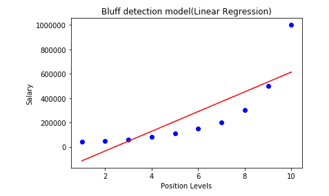
Linear Regression Visualization:
	# Visualizing the Linear Regression results
	plt.scatter(x, y, color='blue')
	plt.plot(x, lin_reg.predict(x), color='red')
	plt.title('Bluff Detection (Linear Regression)')
	plt.xlabel('Position Level')
	plt.ylabel('Salary')
	plt.show()
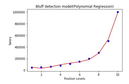
Polynomial Regression Visualization:
	#Visualizing the Polynomial Regression results
	plt.scatter(x, y, color='blue')
	plt.plot(x, lin_reg_2.predict(poly_reg.fit_transform(x)), color='red')
	plt.title('Bluff Detection (Polynomial Regression)')
	plt.xlabel('Position Level')
	plt.ylabel('Salary')
	plt.show()
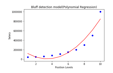
In these visualizations, the Polynomial Regression curve follows the data more closely than the Linear Regression line, indicating better performance for non-linear data.
For degree = 3: When we adjust the degree of the polynomial regression to 3, the resulting plot becomes more accurate, capturing the nuances of the data more effectively. This higher-degree model better reflects the non-linear relationship between position levels and salaries, as demonstrated in the updated plot below.
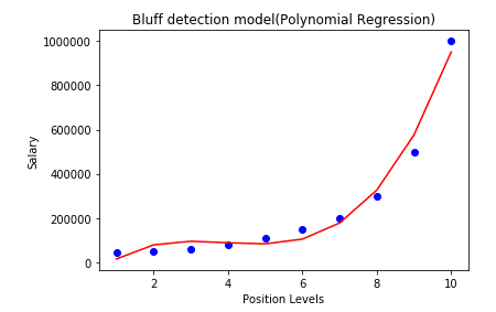
In the plot, the predicted salary for a candidate at level 6.5 is estimated to be in the range of 170K$ to 190K$. This estimation closely aligns with the candidate’s stated salary, suggesting that their claim may be accurate.
Degree = 4: Increasing the degree further to 4 yields an even more precise plot, with the model adapting closely to the data points. This higher-degree polynomial regression provides a more accurate representation of the underlying patterns, allowing for improved predictions. Such adjustments are particularly beneficial when dealing with complex, non-linear datasets, where a more detailed model is needed to capture the variations in the data.
Predicting Results:
	# Predicting with Linear Regression
	linear_prediction = lin_reg.predict([[6.5]])

	# Predicting with Polynomial Regression
	polynomial_prediction = lin_reg_2.predict(poly_reg.fit_transform([[6.5]]))
The Polynomial Regression prediction is closer to the actual value, demonstrating its effectiveness in handling non-linear data.
Conclusion
Polynomial Regression is an essential tool in Machine Learning for modeling non-linear relationships. By adding polynomial terms, it extends the capabilities of linear models and achieves higher accuracy. Understanding how to apply it through Python ensures robust predictions in complex real-world scenarios.