Dimensionality Reduction Technique
In this page, we will learn Dimensionality Reduction Technique, What is Dimensionality Reduction?, The Curse of Dimensionality, Benefits of applying Dimensionality Reduction, Disadvantages of dimensionality Reduction, Approaches of Dimension Reduction, Common techniques of Dimensionality Reduction, Principal Component Analysis (PCA), Backward Feature Elimination, Forward Feature Selection, Missing Value Ratio, Low Variance Filter, High Correlation Filter.
What is Dimensionality Reduction?
Dimensionality refers to the amount of input characteristics, variables, or columns in a dataset, and dimensionality reduction refers to the process of reducing these features.
In some circumstances, a dataset has a large number of input features, making predictive modeling more difficult. Because it is difficult to visualize or forecast a training dataset with a large number of characteristics, dimensionality reduction techniques must be used in such circumstances.
The term "dimensionality reduction technique" refers to the process of reducing the number of dimensions. It can be defined as, "It is a way of converting the higher dimensions dataset into lesser dimensions dataset ensuring that it provides similar information." These methods are commonly utilized in machine learning to develop a more accurate predictive model while solving classification and regression challenges.
Speech recognition, signal processing, bioinformatics, and other fields that deal with high-dimensional data use it frequently. It can also be used to visualize data, reduce noise, and do cluster analysis, among other things.
The Curse of Dimensionality
The curse of dimensionality refers to the difficulty of dealing with high-dimensional data in practice. Any machine learning technique and model becomes increasingly sophisticated as the dimensionality of the input dataset grows. As the number of features grows, the number of samples grows proportionally as well, increasing the risk of overfitting. When a machine learning model is trained on large amounts of data, it becomes overfitted and performs poorly.
As a result, it is frequently necessary to reduce the amount of features, which can be accomplished by dimensionality reduction.
Benefits of applying Dimensionality Reduction
The following are some of the advantages of using a dimensionality reduction technique on a given dataset:
- The space required to store the dataset is lowered by lowering the dimensionality of the features.
- Reduced feature dimensions necessitate less Computation training time.
- The reduced dimensions of the dataset's features aid in quickly displaying the data.
- It takes care of multicollinearity to remove redundant features (if any are present).
Disadvantages of dimensionality Reduction
There are a few drawbacks to using dimensionality reduction, which are listed below:
- Due to the reduction in dimensionality, some data may be lost.
- The principal components that must be considered in the PCA dimensionality reduction technique are occasionally unknown.
Approaches of Dimension Reduction
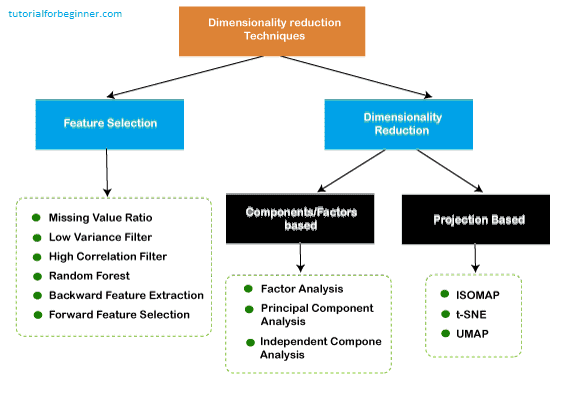
There are two ways to apply the dimension reduction technique, which are given below:
Feature Selection
To develop a high-accuracy model, feature selection is the process of picking a subset of important characteristics and excluding irrelevant features from a dataset. In other words, it's a method for choosing the best characteristics from a dataset.
The feature selection is done in three ways:
-
Filters Methods
The dataset is filtered in this manner, and only the relevant features are taken as a subset. The following are some examples of filtering techniques:
- Correlation
- Chi-Square Test
- ANOVA
- Information Gain, etc.
-
Wrappers Methods
The wrapper method achieves the same aim as the filter function, but it evaluates it using a machine learning model. In this procedure, various features are fed into the machine learning model, and the performance is evaluated. To improve the model's accuracy, the performance selects whether to include or eliminate those features. This method is more accurate than filtering, but it is more difficult to implement. The following are some examples of wrapper methods:
- Forward Selection
- Backward Selection
- Bi-directional Elimination
-
Embedded Methods:
Methods that are embedded Examine the machine learning model's several training iterations and rank the value of each feature. Embedded methods are used in a variety of ways, including:
- LASSO
- Elastic Net
- Ridge Regression, etc.
Feature Extraction:
The process of changing a space with many dimensions into a space with fewer dimensions is known as feature extraction. This method is handy when we want to keep all of the information while processing it with fewer resources.
Some common feature extraction techniques are:
- Principal Component Analysis
- Linear Discriminant Analysis
- Kernel PCA
- Quadratic Discriminant Analysis
Common techniques of Dimensionality Reduction
- Principal Component Analysis
- Backward Elimination
- Forward Selection
- Score comparison
- Missing Value Ratio
- Low Variance Filter
- High Correlation Filter
- Random Forest
- Factor Analysis
- Auto-Encoder
Principal Component Analysis (PCA)
With the use of orthogonal transformation, Principal Component Analysis turns the observations of correlated characteristics into a set of linearly uncorrelated features. The Principal Components are the newly altered features. It's one of the most widely used programs for exploratory data analysis and predictive modeling.
The variance of each characteristic is taken into account by PCA since the high attribute indicates a good separation between the classes and so minimizes dimensionality. Image processing, movie recommendation systems, and optimizing power allocation in multiple communication channels are some of the real-world uses of PCA.
Backward Feature Elimination
When creating a Linear Regression or Logistic Regression model, the backward feature elimination strategy is commonly utilized. The following steps are used in this strategy to reduce dimensionality or select features:
- To begin, all n variables from the given dataset are used to train the model in this method.
- The model's performance is examined.
- Now we'll eliminate one feature at a time and train the model on n-1 features for n times before calculating the model's performance.
- We'll look for the variable that has had the smallest or no effect on the model's performance, and then we'll remove that variable or features, leaving us with n-1 features.
- Rep the procedure till no more features can be dropped.
We can specify the ideal amount of features required for machine learning algorithms using this strategy, which involves picking the best model performance and the highest tolerable error rate.
Forward Feature Selection
The backward elimination method is reversed in the forward feature selection phase. It indicates that in this strategy, we won't remove a feature; instead, we'll locate the greatest characteristics that will boost the model's performance the most. This approach involves the following steps:
- We will begin with a single feature and gradually add each feature one at a time.
- We'll train the model on each feature separately in this section.
- The feature that performs the best is chosen.
- The approach will be continued until the model's performance has significantly improved.
Missing Value Ratio
If there are too many missing values in a dataset, we remove those variables because they don't provide much information. To do this, we may specify a threshold level, and if a variable has more missing values than that threshold, the variable will be dropped. The more efficient the reduction, the higher the threshold value.
Low Variance Filter
Data columns with certain changes in the data have less information, just like the missing value ratio technique. As a result, we must calculate the variance of each variable, and all data columns with variance less than a certain threshold must be removed, as low variance characteristics will have no effect on the target variable.
High Correlation Filter
When two variables provide essentially similar information, this is referred to be high correlation. The model's performance may be harmed as a result of this factor. The estimated value of the correlation coefficient is based on the correlation between the independent numerical variables. We can eliminate one of the variables from the dataset if this value is higher than the threshold value. Those factors or traits with a high correlation with the target variable can be considered.
Random Forest
In machine learning, Random Forest is a common and helpful feature selection approach. We don't need to program the feature importance package separately because this method has one built in. In this strategy, we need to create a huge number of trees against the target variable, and then locate the subset of features using usage statistics for each attribute.
Because the random forest technique uses only numerical variables, we must use hot encoding to convert the input data to numeric data.
Factor Analysis
Factor analysis is a technique in which each variable is kept within a group according to the correlation with other variables, it means variables within a group can have a high correlation between themselves, but they have a low correlation with variables of other groups.
For example, if we have two variables, Income and Spend, we can grasp it. These two factors are highly correlated, implying that those with higher income spend more, and vice versa. As a result, similar variables are grouped together, and that group is referred to as the factor. In comparison to the dataset's original dimension, the number of these factors will be reduced.
Auto-encoders
The auto-encoder, which is a sort of ANN or artificial neural network with the goal of copying inputs to outputs, is one of the most prominent methods of dimensionality reduction. This compresses the input into a latent-space representation, which is then used to produce the output. It is divided into two sections:
Encoder: The encoder's job is to compress the input so that the latent-space representation may be formed.
Decoder: The decoder's job is to reconstruct the output from the latent-space representation.