Multiple Linear Regression in Machine Learning

In this page, we will learn What is Multiple Linear Regression in Machine Learning?, Some key points about MLR, MLR equation, Assumptions for Multiple Linear Regression, Implementation of Multiple Linear Regression model using Python, Applications of Multiple Linear Regression.

---

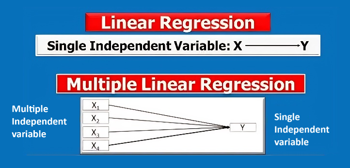
What is Multiple Linear Regression in Machine Learning?

We learned about Simple Linear Regression in the previous topic, where a single Independent/Predictor(X) variable is utilized to model the response variable (Y). However, there are some circumstances where more than one predictor variable affects the response variable; in these cases, the Multiple Linear Regression technique is applied.

Furthermore, Multiple Linear Regression is an extension of Simple Linear Regression in that it predicts the response variable using more than one predictor variable. It can be defined as follows:

“Multiple Linear Regression is one of the important regression algorithms which models the linear relationship between a single dependent continuous variable and more than one independent variable.”

Example:
Prediction of CO2 emission based on engine size and number of cylinders in a car.

Some key points about MLR:

• The dependent or target variable (Y) must be continuous/real for MLR to work, although the predictor or independent variable might be continuous or categorical.
• Each feature variable must model the dependent variable's linear connection.
• MLR is a technique for fitting a regression line through a multidimensional space of data points.

In this step, we'll build a Simple Linear Regression model to determine which line best represents the relationship between these two variables.

To use Python to create the Simple Linear regression model in machine learning, follow the steps below:

MLR equation:

The target variable (Y) in Many Linear Regression is a linear mixture of multiple predictor variables x1, x2, x3,...,xn. The equation becomes: Since it is an upgrade of Simple Linear Regression, the same is done to the multiple linear regression equation.
Y= b₀+b₁x₁+ b₂x₂+ b₃x₃+...... b_nx_n ............... (a)

Where,
Y= Output/Response variable
b₀, b₁, b₂, b₃ , b_n....= Coefficients of the model.
x₁, x₂, x₃, x₄,...= Various Independent / feature variable

Assumptions for Multiple Linear Regression:

• The Target and Predictor variables should have a linear relationship.
• The residuals from the regression must be normally distributed.
• MLR considers data to have minimal or no multicollinearity (correlation between independent variables).

Implementation of Multiple Linear Regression model using Python:

To implement MLR using Python, we have below problem:

Problem Description:

We have 50 start-up companies in our database. R&D Spend, Administration Spend, Marketing Spend, State, and Profit for a financial year are all included in this dataset. Our goal is to develop a model that can quickly assess which company has the highest profit margin and which element has the most impact on a company's profit margin.

Profit is the dependent variable, and the other four variables are independent variables, because we need to find it. The following are the key phases in implementing the MLR model:

• Data Pre-processing Steps
• Fitting the MLR model to the training set
• Predicting the result of the test set

Step-1: Data Pre-processing Step:

Data pre-processing is the initial phase, which we've already covered in this course. The steps in this procedure are as follows:

• Importing libraries: We'll start by importing the library that will assist us in creating the model. The code for it is as follows:
  

 
  #importing libraries 
  import numpy as nm  
  import matplotlib.pyplot as mtp 
  import pandas as pd 

• Importing dataset: We'll now import the 50 CompList dataset, which contains all of the variables. The code for it is as follows:
  
  

  #importing datasets 
  data_set = pd.read_csv('50_CompList.csv')  

Output: We will get the dataset as:

We can see that there are five variables in the above output, four of which are continuous and one of which is categorical.

• Extracting dependent and independent Variables:

    #Extracting Independent and dependent Variable
    x = data_set.iloc[:, :-1].values 
    y = data_set.iloc[:, 4].values 

Output:

Out[5]:

  array([[165349.2, 136897.8, 471784.1, 'New York'],
    [162597.7, 151377.59, 443898.53, 'California'],
    [153441.51, 101145.55, 407934.54, 'Florida'],
    [144372.41, 118671.85, 383199.62, 'New York'],
    [142107.34, 91391.77, 366168.42, 'Florida'],
    [131876.9, 99814.71, 362861.36, 'New York'],
    [134615.46, 147198.87, 127716.82, 'California'],
    [130298.13, 145530.06, 323876.68, 'Florida'],
    [120542.52, 148718.95, 311613.29, 'New York'],
    [123334.88, 108679.17, 304981.62, 'California'],
    [101913.08, 110594.11, 229160.95, 'Florida'],
    [100671.96, 91790.61, 249744.55, 'California'],
    [93863.75, 127320.38, 249839.44, 'Florida'],
    [91992.39, 135495.07, 252664.93, 'California'],
    [119943.24, 156547.42, 256512.92, 'Florida'],
    [114523.61, 122616.84, 261776.23, 'New York'],
    [78013.11, 121597.55, 264346.06, 'California'],
    [94657.16, 145077.58, 282574.31, 'New York'],
    [91749.16, 114175.79, 294919.57, 'Florida'],
    [86419.7, 153514.11, 0.0, 'New York'],
    [76253.86, 113867.3, 298664.47, 'California'],
    [78389.47, 153773.43, 299737.29, 'New York'],
    [73994.56, 122782.75, 303319.26, 'Florida'],
    [67532.53, 105751.03, 304768.73, 'Florida'],
    [77044.01, 99281.34, 140574.81, 'New York'],
    [64664.71, 139553.16, 137962.62, 'California'],
    [75328.87, 144135.98, 134050.07, 'Florida'],
    [72107.6, 127864.55, 353183.81, 'New York'],
    [66051.52, 182645.56, 118148.2, 'Florida'],
    [65605.48, 153032.06, 107138.38, 'New York'],
    [61994.48, 115641.28, 91131.24, 'Florida'],
    [61136.38, 152701.92, 88218.23, 'New York'],
    [63408.86, 129219.61, 46085.25, 'California'],
    [55493.95, 103057.49, 214634.81, 'Florida'],
    [46426.07, 157693.92, 210797.67, 'California'],
    [46014.02, 85047.44, 205517.64, 'New York'],
    [28663.76, 127056.21, 201126.82, 'Florida'],
    [44069.95, 51283.14, 197029.42, 'California'],
    [20229.59, 65947.93, 185265.1, 'New York'],
    [38558.51, 82982.09, 174999.3, 'California'],
    [28754.33, 118546.05, 172795.67, 'California'],
    [27892.92, 84710.77, 164470.71, 'Florida'],
    [23640.93, 96189.63, 148001.11, 'California'],
    [15505.73, 127382.3, 35534.17, 'New York'],
    [22177.74, 154806.14, 28334.72, 'California'],
    [1000.23, 124153.04, 1903.93, 'New York'],
    [1315.46, 115816.21, 297114.46, 'Florida'],
    [0.0, 135426.92, 0.0, 'California'],
    [542.05, 51743.15, 0.0, 'New York'],
    [0.0, 116983.8, 45173.06, 'California']], dtype=object)

As can be seen in the result above, the last column comprises categorical variables that are not suitable for fitting the model directly. As a result, we must encrypt this variable.

Encoding Dummy Variables:

We will encode one categorical variable (State) because it cannot be directly applied to the model. The LabelEncoder class will be used to convert the categorical variable to integers. However, it is insufficient because there is still some relational order, which may result in an incorrect model. To solve this problem, we'll employ OneHotEncoder, which will generate dummy variables. The following is the code for it:

  #Catgorical data  
  from sklearn.preprocessing import LabelEncoder,OneHotEncoder
  labelencoder_x = LabelEncoder()
  x[:, 3] = labelencoder_x.fit_transform(x[:,3])
  onehotencoder = OneHotEncoder(categorical_features = [3])
  x = onehotencoder.fit_transform(x).toarray()  

Because the other variables are continuous, we are only encoding one independent variable, which is state.

Output:

The state column has been turned into dummy variables, as shown in the above output (0 and 1). Each dummy variable column corresponds to a single State in this example. By comparing it to the original dataset, we can be sure. The first column corresponds to the state of California, the second column to the state of Florida, and the third column to the state of New York.

[ Note: We should not use all of the dummy variables at the same time, thus the number of dummy variables must be 1 fewer than the total number of dummy variables; otherwise, a dummy variable trap will result. ]

• To avoid the dummy variable trap, we're creating a single line of code now:
  

 
  #avoiding the dummy variable trap: 
  x = x[:, 1:]

It's possible that if we don't delete the first dummy variable, the model will become multicollinear.

The first column has been eliminated, as seen in the output image above.

We'll now divide the dataset into two groups: training and testing. The following is the code for this:

 
  #Splitting the dataset into training and test set. 
  from sklearn.model_selection import train_test_split 
  x_train, x_test, y_train, y_test = train_test_split( x, y,test_size = 0.2, random_state = 0 ) 

The above code will split our dataset into a training set and test set.
The preceding code will partition the dataset into two sets: training and test. The output can be viewed by using the variable explorer option in Spyder IDE, which will display the test and training sets as shown below:

Training set:

Note: We will not implement feature scaling in MLR because the library will take care of it and we won't have to do it manually.

Step: 2- Fitting our MLR model to the Training set:

Now that our dataset has been properly prepared for training, we will fit our regression model to the training set. It will be identical to the Simple Linear Regression model that we used previously. This will be coded as follows:

 
  #Fitting the MLR model to the training set:
  from sklearn.linear_model import LinearRegression 
  regressor = LinearRegression() 	
  regressor.fit(x_train, y_train) 	

Output:
Out[9]: LinearRegression(copy_X=True, fit_intercept=True, n_jobs=None, normalize=False)
Using the training dataset, we've effectively trained our model. We'll use the test dataset to evaluate the model's performance in the next phase.

Step: 3- Prediction of Test set results:

The final step in our model's development is to evaluate its performance. We'll do it by forecasting the outcome of the test set. A y_pred vector will be created for prediction. The code for it is as follows:

 
  #Predicting the Test set result; 
  y_pred = regressor.predict(x_test)

Output:

We have anticipated result set and test set in the above output. By comparing these two values index by index, we may evaluate the model's performance. The first index, for example, has predicted profit of 103015 dollars and a test/real profit of 103282 dollars. The difference is only 267 dollars, which is a good prediction, thus our model is completely complete.

We may also look at the scores for the training and test datasets. The code for it is as follows:

 
  print('Train Score: ', regressor.score(x_train, y_train))
  print('Test Score: ', regressor.score(x_test, y_test))                               

Output: The score is:

 
  Train Score: 0.9501847627493607
  Test Score: 0.9347068473282446									

Our model is 95 percent accurate with the training dataset and 93 percent accurate with the test dataset, according to the above score.
Note: In the next article, we'll look at how we may use the Backward Elimination procedure to improve the model's performance.

Applications of Multiple Linear Regression:

Multiple Linear Regression has primarily two applications:

• Effectiveness of Independent variable on prediction:
• Predicting the impact of changes: