Backward Elimination in ML
Table of Contents:
- What is Backward Elimination?
- The Process of Backward Elimination
- Real-World Use Case
- Benefits of Backward Elimination
- Comparison with Other Methods
- Step-by-Step Implementation in Python
- Automating Backward Elimination
- Cross-Validation for Model Evaluation
- Conclusion
Content Highlight:
This comprehensive guide on Backward Elimination explains the step-by-step process used to remove insignificant features in a Multiple Linear Regression model, improving accuracy and performance. It highlights the benefits of backward elimination, such as better interpretability and efficiency, compared to other feature selection methods like Forward Selection and Stepwise Selection. Using the 50_Startups dataset, the guide includes detailed Python code for implementation, automating the process, and validating model performance with cross-validation. It also covers real-world applications and provides additional insights into handling multicollinearity with a correlation heatmap. Overall, this guide equips readers with the tools to build optimized regression models.
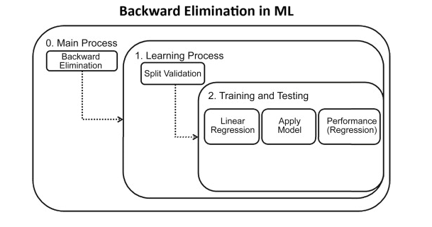
What is Backward Elimination?
Backward Elimination is a step-by-step process used to remove features that don't significantly contribute to the prediction of the dependent variable. Compared to other model-building methods like Forward Selection or Bidirectional Elimination, Backward Elimination is fast, efficient, and ensures that only the most important variables remain.
The Process of Backward Elimination
Step-by-Step Guide:
- Step 1: Define a significance level (SL), typically 0.05. This threshold will guide which variables are retained or eliminated.
- Step 2: Fit the full model with all available independent variables to start with the most comprehensive version.
- Step 3: Check the P-values for all predictors. Identify the variable with the highest P-value. If P > SL, proceed to the next step. If P ≤ SL, the process ends, and your final model is ready.
- Step 4: Remove the predictor with the highest P-value.
- Step 5: Refit the model with the remaining variables and repeat the process until only significant variables remain (P ≤ SL).
Real-World Use Case of Backward Elimination:
Let's consider an example where a company wants to predict profit based on multiple factors like R&D expenditure, marketing spend, and state location. The company can use Backward Elimination to remove irrelevant factors that don’t significantly impact the prediction, allowing them to focus on the key drivers of profit.
Benefits of Backward Elimination:
- Improved Interpretability: A model with fewer variables is easier to understand and explain.
- Increased Efficiency: A leaner model with fewer variables is faster to run and easier to maintain.
- Better Predictions: By focusing on the most significant features, the model makes more accurate predictions.
Comparison of Feature Selection Methods:
| Method | Description | Strengths | Weaknesses |
|---|---|---|---|
| Backward Elimination | Starts with all features, removes the least significant one step-by-step. | Ensures that only the most significant features are retained. | Can be computationally expensive with many features. |
| Forward Selection | Starts with no features, adds the most significant one step-by-step. | Fast for large datasets with few significant predictors. | May miss feature interactions. |
| Stepwise Selection | Combines Forward and Backward Elimination approaches. | Balances accuracy and efficiency. | More complex and computationally expensive. |
Backward Elimination: Step-by-Step Implementation in Python
This guide walks through the process of Backward Elimination, a feature selection technique for building optimal regression models. We will use the 50_Startups dataset for this demonstration. Each step is explained in detail, including Python code implementation.
Step 1: Importing Necessary Libraries
We first need to import the necessary libraries:
numpyandpandasare used for data manipulation.statsmodels.apiprovides the function to perform Ordinary Least Squares (OLS) regression, which we will use for backward elimination.sklearnprovides utility functions like label encoding and train-test splitting.
   import numpy as np
   import pandas as pd
   import statsmodels.api as sm
   from sklearn.model_selection import train_test_split
   from sklearn.preprocessing import LabelEncoder, OneHotEncoder
   from sklearn.compose import ColumnTransformer
Step 2: Loading the Dataset
We will load the Download 50_Startups Dataset into a Pandas DataFrame. The dataset contains information about different startups, including their R&D, administration, and marketing expenses, and their profit.
   # Load the dataset
   dataset = pd.read_csv('50_Startups.csv')

   # Display the first few rows of the dataset
   print(dataset.head())
Step 3: Data Preprocessing
We need to encode the categorical data, in this case, the "State" column. This column has three states (California, Florida, and New York), which we will encode as dummy variables using OneHotEncoder. We will also avoid the "dummy variable trap" by removing one of the dummy variables.
   # Separate features (independent variables) and target (dependent variable)
   X = dataset.iloc[:, :-1].values  # All columns except the last one (Profit)
   y = dataset.iloc[:, -1].values   # The last column (Profit)

   # Encoding the categorical data (State)
   labelencoder = LabelEncoder()
   X[:, 3] = labelencoder.fit_transform(X[:, 3])  # Encode the "State" column

   # One-hot encoding to convert state into dummy variables
   ct = ColumnTransformer([('encoder', OneHotEncoder(), [3])], remainder='passthrough')
   X = np.array(ct.fit_transform(X))

   # Avoid the dummy variable trap by removing one dummy variable
   X = X[:, 1:]
Correlation Heatmap
Before applying Backward Elimination, it's useful to visualize the correlation between variables to identify multicollinearity, which can affect the regression model.
Step 4: Adding the Intercept Term
In regression models, an intercept term is required. This is why we add a column of ones to represent the intercept term for our regression equation.
   # Add a column of ones to the matrix X for the intercept term
   X = np.append(arr=np.ones((50, 1)).astype(int), values=X, axis=1)
Step 5: Backward Elimination
We begin backward elimination by fitting the model with all predictors. Then, we look at the P-values for each predictor, removing the predictor with the highest P-value if it is greater than the significance level (usually 0.05).
   # Step 1: Fit the full model with all predictors
   X_opt = X[:, :]  # Start with all predictors
   regressor_OLS = sm.OLS(endog=y, exog=X_opt).fit()  # Ordinary Least Squares regression
   print(regressor_OLS.summary())
Automating Backward Elimination:
We can automate the backward elimination process by defining a Python function that removes variables based on their P-values.
    def backward_elimination(X, y, sl):
        numVars = len(X[0])
        for i in range(0, numVars):
            regressor_OLS = sm.OLS(y, X).fit()
            maxPVal = max(regressor_OLS.pvalues)
            if maxPVal > sl:
                for j in range(0, numVars - i):
                    if (regressor_OLS.pvalues[j] == maxPVal):
                        X = np.delete(X, j, 1)
        regressor_OLS.summary()
        return X

    SL = 0.05
    X_opt = backward_elimination(X, y, SL)
Cross-Validation for Model Evaluation:
After applying Backward Elimination, it is important to evaluate the model's performance using cross-validation. This method ensures the model generalizes well to new data and avoids overfitting.
   from sklearn.model_selection import cross_val_score
   accuracies = cross_val_score(estimator = regressor_OLS, X = X_train, y = y_train, cv = 10)
   print("Accuracy: {:.2f} %".format(accuracies.mean()*100))
   print("Standard Deviation: {:.2f} %".format(accuracies.std()*100))
Conclusion:
Backward Elimination is a crucial technique for improving model performance by removing irrelevant predictors. By reducing model complexity, you can achieve higher accuracy and better interpretability. Whether you're building a predictive model for marketing analysis, financial forecasting, or any other domain, Backward Elimination can help ensure that only the most significant features remain in your model.
- Start with all features, remove the least significant one by one.
- Check P-values after each iteration and remove features with P-values > 0.05.
- Cross-validate the final model to ensure generalization to unseen data.