Naive Bayes Classifier Algorithm in Machine Learning

In this page, we will learn What is Naive Bayes Classifier Algorithm in machine learning?, Why is it called Naive Bayes?, Bayes Theorem, Frequency table for the Weather Conditions, Likelihood table weather condition, Advantages of Naive Bayes Classifier, Disadvantages of Naive Bayes Classifier, Applications of Naive Bayes Classifier, Types of Naive Bayes Model.

What is Naive Bayes Classifier Algorithm in machine learning?

The Nave Bayes algorithm is a supervised learning algorithm for addressing classification issues that is based on the Bayes theorem.
It is mostly utilized in text classification tasks that require a large training dataset.
The Nave Bayes Classifier is a simple and effective classification method that aids in the development of fast machine learning models capable of making quick predictions.
It's a probabilistic classifier, which means it makes predictions based on an object's probability.
Spam filtration, sentiment analysis, and article classification are all common uses of the Nave Bayes Algorithm.

Why is it called Naive Bayes?

The two words Nave and Bayes make up the Nave Bayes algorithm, which can be described as:

Naïve: It's termed Nave because it assumes that the appearance of one feature is unrelated to the appearance of other features. If the color, shape, and flavor of the fruit are used to identify it, a red, spherical, and sweet fruit is identified as an apple. As a result, each feature contributes to identifying that it is an apple without relying on the others.
Bayes: It's called Bayes because it's based on the Bayes' Theorem principle

Bayes' Theorem:

Bayes' theorem, often known as Bayes' Rule or Bayes' law, is a mathematical formula for calculating the probability of a hypothesis given previous information. It is conditional probability that determines this.
The Bayes theorem's formula is as follows:

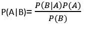
Where,
P(A|B) is Posterior probability: Probability of hypothesis A on the observed event B.
P(B|A) is Likelihood probability: Probability of the evidence given that the probability of a hypothesis is true.
P(A) is Prior Probability: Probability of hypothesis before observing the evidence.
P(B) is Marginal Probability: Probability of Evidence.

Working of Naïve Bayes' Classifier:
Assume we have a dataset of weather conditions and a goal variable called "Play." So, utilizing this dataset, we must select whether or not to play on a specific day based on the weather circumstances. To fix this problem, we must take the following steps:

Create frequency tables from the given dataset.
Find the probability of given features to generate a Likelihood table.
Calculate the posterior probability using Bayes' theorem.

Problem: Should the Player play or not play if the weather is sunny?
Solution: To begin, examine the following dataset:

	Outlook	Play
0	Rainy	Yes
1	Sunny	Yes
2	Overcast	Yes
3	Overcast	Yes
4	Sunny	No
5	Rainy	Yes
6	Sunny	Yes
7	Overcast	Yes
8	Rainy	No
9	Sunny	No
10	Sunny	Yes
11	Rainy	No
12	Overcast	Yes
13	Overcast	Yes

Frequency table for the Weather Conditions:

Weather	Yes	No
Overcast	5	0
Rainy	2	2
Sunny	3	2
Total	10	0

Likelihood table weather condition:

Weather	No	Yes
Overcast	0	5	5/14= 0.35
Rainy	2	2	4/14=0.29
Sunny	2	3	5/14=0.35
All	4/14=0.29	10/14=0.71

Advantages of Naive Bayes Classifier:

Nave Bayes is a fast and simple machine learning algorithm for predicting a class of datasets.
It's suitable for both binary and multi-class classifications.
In comparison to the other Algorithms, it performs better in Multi-class predictions.
It is the most often used method for text classification problems.

Disadvantages of Naive Bayes Classifier:

Because Naive Bayes implies that all features are unrelated or independent, it is unable to learn the link between them.

Applications of Naive Bayes Classifier:

It is used for Credit Scoring.
It is used in medical data classification.
It can be used in real-time predictions because Naïve Bayes Classifier is an eager learner.
It is used in Text classification such as Spam filtering and Sentiment analysis.

Types of Naive Bayes Model:

There are three different forms of Naive Bayes Models, as listed below:

Gaussian: The Gaussian model assumes that features are distributed in a regular manner. If predictors take continuous values rather than discrete values, the model assumes that these values are drawn from a Gaussian distribution.
Multinomial: When the data is multinomial distributed, the Multinomial Nave Bayes classifier is utilized. It is primarily used to solve document classification issues, which involves determining which category a document belongs to, such as Sports, Politics, or Education.
The predictions in the classifier are based on the frequency of term
Bernoulli: Like the Multinomial classifier, the Bernoulli classifier uses independent Booleans variables as predictor variables. For example, determining whether or not a specific word appears in a document. This paradigm is also well-known for jobs involving document classification.

Python Implementation of the Naive Bayes algorithm:

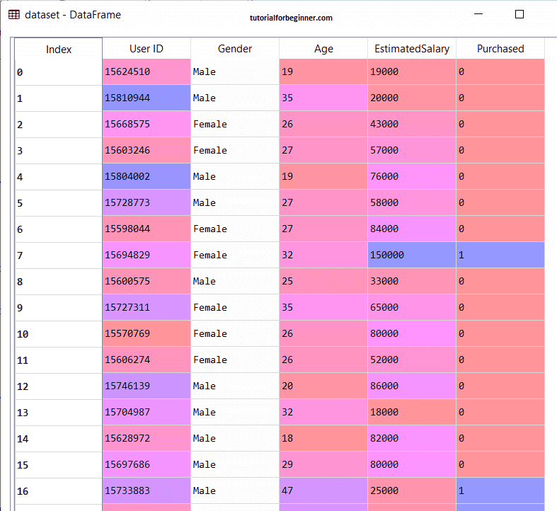
Now we'll use Python to create a Naive Bayes Algorithm. As a result, we'll use the "user data" dataset, which we previously employed in our classification model. As a result, comparing the Naive Bayes model to the other models is simple.

Steps to implement:

Data Pre-processing step
Fitting Logistic Regression to the Training set
Predicting the test result
Test accuracy of the result(Creation of Confusion matrix)
Visualizing the test set result.

1. Data Pre-processing step:

We'll pre-process/prepare the data in this stage so that we can use it effectively in our code. It's the same thing we accomplished with data pre-processing. The following is the code for this:

 
  Importing the libraries  
  import numpy as nm  
  import matplotlib.pyplot as mtp  
  import pandas as pd  
    
  #Importing the dataset  
  dataset = pd.read_csv('user_data.csv')  
  x = dataset.iloc[:, [2, 3]].values  
  y = dataset.iloc[:, 4].values  
    
  #Splitting the dataset into the Training set and Test set  
  from sklearn.model_selection import train_test_split  
  x_train, x_test, y_train, y_test = train_test_split(x, y, test_size = 0.25, random_state = 0)  
    
  #Feature Scaling  
  from sklearn.preprocessing import StandardScaler  
  sc = StandardScaler()  
  x_train = sc.fit_transform(x_train)  
  x_test = sc.transform(x_test)

"dataset = pd.read csv('user data.csv')" was used to load the dataset into our program in the previous code. After dividing the loaded dataset into training and test sets, we scaled the feature variable.

The output for the dataset is given as:

2) Fitting Naive Bayes to the Training Set:

We'll now fit the Naive Bayes model on the Training set after the pre-processing step. The code for it is as follows:

 
  #Fitting Naive Bayes to the Training set  
  from sklearn.naive_bayes import GaussianNB  
  classifier = GaussianNB()  
  classifier.fit(x_train, y_train)

We utilized the GaussianNB classifier to fit it to the training dataset in the preceding code. Other classifiers can also be used depending on our needs.

Output:

Output:

 
  Out[6]: GaussianNB(priors = None, var_smoothing = 1e-09)

3) Prediction of the test set result:

Now we'll forecast the outcome of the test set. To do so, we'll make predictions using the predict function and a new predictor variable called y_pred.

 
  # Predicting the Test set results  
  y_pred = classifier.predict(x_test)

Output:

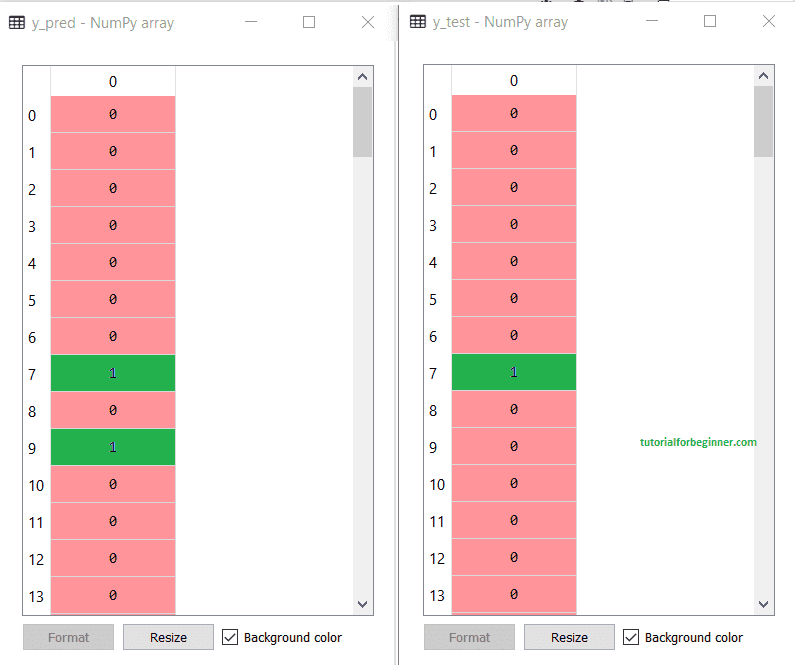
The output for prediction vector y_pred and real vector y_test is shown above. We can observe that certain projections differ from the actual numbers, indicating that they are erroneous.

4) Creating Confusion Matrix:

The Confusion matrix will now be used to test the accuracy of the Naive Bayes classifier. The code for it is as follows:

 
  # Making the Confusion Matrix  
  from sklearn.metrics import confusion_matrix  
  cm = confusion_matrix(y_test, y_pred)

Output:

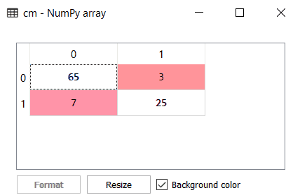
As we can see in the above confusion matrix output, there are 7 + 3 = 10 incorrect predictions, and 65+25=90 correct predictions.

5) Visualizing the training set result:

The training set result will then be visualized using the Nave Bayes Classifier. The code for it is as follows:

 
  # Visualising the Training set results  
  from matplotlib.colors import ListedColormap  
  x_set, y_set = x_train, y_train  
  X1, X2 = nm.meshgrid(nm.arange(start = x_set[:, 0].min() - 1, stop = x_set[:, 0].max() + 1, step = 0.01),  
                        nm.arange(start = x_set[:, 1].min() - 1, stop = x_set[:, 1].max() + 1, step = 0.01))  
  mtp.contourf(X1, X2, classifier.predict(nm.array([X1.ravel(), X2.ravel()]).T).reshape(X1.shape),  
              alpha = 0.75, cmap = ListedColormap(('purple', 'green')))  
  mtp.xlim(X1.min(), X1.max())  
  mtp.ylim(X2.min(), X2.max())  
  for i, j in enumerate(nm.unique(y_set)):  
    mtp.scatter(x_set[y_set == j, 0], x_set[y_set == j, 1],  
      c = ListedColormap(('purple', 'green'))(i), label = j)  
  mtp.title('Naive Bayes (Training set)')  
  mtp.xlabel('Age')  
  mtp.ylabel('Estimated Salary')  
  mtp.legend()  
  mtp.show()

Output:

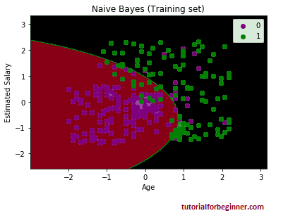
We can observe that the Nave Bayes classifier has separated the data points with the fine boundary in the above output. We used the GaussianNB classifier in our algorithm, therefore it's a Gaussian curve.image.

6) Visualizing the Test set result:

 
  #Visualising the Test set results  
  from matplotlib.colors import ListedColormap  
  x_set, y_set = x_test, y_test  
  X1, X2 = nm.meshgrid(nm.arange(start = x_set[:, 0].min() - 1, stop = x_set[:, 0].max() + 1, step = 0.01),  
                       nm.arange(start = x_set[:, 1].min() - 1, stop = x_set[:, 1].max() + 1, step = 0.01))  
  mtp.contourf(X1, X2, classifier.predict(nm.array([X1.ravel(), X2.ravel()]).T).reshape(X1.shape),  
              alpha = 0.75, cmap = ListedColormap(('purple', 'green')))  
  mtp.xlim(X1.min(), X1.max())  
  mtp.ylim(X2.min(), X2.max())  
  for i, j in enumerate(nm.unique(y_set)):  
    mtp.scatter(x_set[y_set == j, 0], x_set[y_set == j, 1],  
      c = ListedColormap(('purple', 'green'))(i), label = j)  
  mtp.title('Naive Bayes (test set)')  
  mtp.xlabel('Age')  
  mtp.ylabel('Estimated Salary')  
  mtp.legend()  
  mtp.show()

Output:

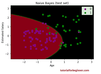
The output seen above is the final result for the test set data. As can be seen, the classifier used a Gaussian curve to split the variables "bought" and "not purchased." In the Confusion matrix, we have derived some incorrect predictions. Nonetheless, it is a decent classifier.