Data Preprocessing for ML
Table of Content:
- Data Preprocessing in Machine Learning: A Comprehensive Guide
- Why is Data Preprocessing Important?
- Key Steps in Data Preprocessing
- Conclusion
Content highlight:
Data preprocessing is the cornerstone of successful machine learning models. It involves transforming raw, noisy, and incomplete data into a refined format, allowing machine learning algorithms to produce accurate and efficient results. This guide delves into critical preprocessing steps, including handling missing data, encoding categorical variables, and feature scaling. You’ll learn how to import essential libraries like NumPy, Pandas, and Scikit-learn, load datasets, and split them into training and testing sets to avoid overfitting. By the end of this guide, you'll have a complete understanding of how to clean and prepare your data to build a robust, high-performing machine learning model, with all steps demonstrated in Python.
Data Preprocessing in Machine Learning: A Comprehensive Guide
Data preprocessing is the cornerstone of any machine learning project. It transforms raw, messy data into a refined format, making it suitable for machine learning models to deliver accurate and efficient results.
In real-world scenarios, datasets are rarely clean. They may be rife with missing values, noise, or inconsistencies. Without proper data preprocessing, these issues can hinder the performance of even the most advanced algorithms. Therefore, ensuring clean, structured, and relevant data is crucial for boosting model accuracy and efficiency.
Why is Data Preprocessing Important?
Machine learning models thrive on high-quality data. Real-world datasets are often imperfect, containing noise, incomplete entries, or irrelevant details. Data preprocessing addresses these issues by transforming raw data into a usable format. This critical step not only improves model performance but also ensures that your model can make reliable predictions. Properly preprocessed data leads to faster, more accurate outcomes, directly impacting the success of your machine learning projects.
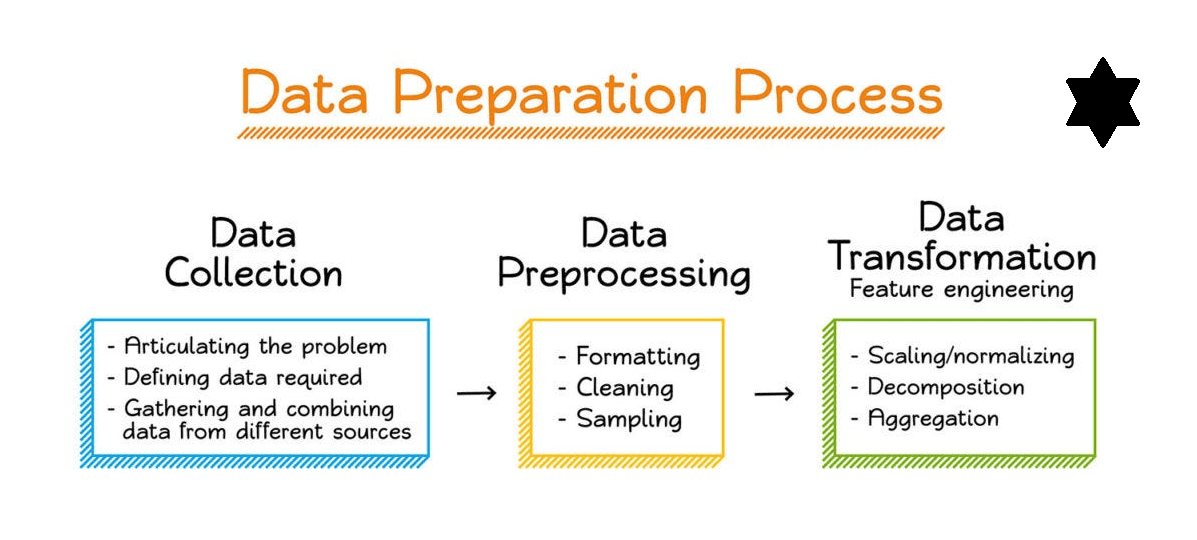
Key Steps in Data Preprocessing:
- Importing Libraries: Use essential Python libraries like NumPy, Pandas, and Scikit-learn to handle data efficiently.
- Acquiring the Dataset: Obtain the raw data, often in the form of CSV files, databases, or other formats.
- Loading the Dataset: Load your data into a suitable structure (such as a DataFrame) to begin cleaning and analysis.
- Handling Missing Data: Deal with incomplete data by filling missing values, removing rows, or applying other imputation techniques.
- Encoding Categorical Variables: Convert non-numeric categorical data into numerical form, using techniques like One-Hot Encoding or Label Encoding, to make it understandable for algorithms.
- Splitting Data into Training and Testing Sets: Divide the dataset into training and testing subsets to ensure the model generalizes well to unseen data.
- Feature Scaling: Normalize or standardize numerical features so they fall within a similar range, enhancing the model's performance and convergence speed.
In summary, data preprocessing is essential to improve the accuracy, speed, and overall efficiency of machine learning models. By following a structured process, you ensure that your model performs optimally with clean, well-structured data.
This comprehensive approach to data preprocessing not only addresses practical challenges but also enhances the likelihood of building a highly accurate and reliable machine learning model.
1. Importing Libraries
Before working with the dataset, you'll need to import the essential libraries that facilitate data manipulation and preprocessing. These libraries include:
- NumPy: For handling arrays and performing numerical computations.
- Pandas: For data manipulation and analysis.
- Matplotlib: For data visualization.
- Scikit-learn: For machine learning preprocessing and algorithms.
    !pip install tensorflow pandas matplotlib //if not installed
    import numpy as np
    import pandas as pd
    import matplotlib.pyplot as plt
    from sklearn.model_selection import train_test_split
    from sklearn.preprocessing import StandardScaler, OneHotEncoder
2. Acquiring the Dataset
The first and most crucial step in any machine learning project is acquiring the dataset. We discussed earlier what a dataset is and where you can source them, so here, we focus on how to load the dataset for your machine learning project.
Typically, datasets are stored in CSV (Comma-Separated Values) files. CSV files are widely used due to their simplicity in storing tabular data. For example:
    Country, Age, Salary, Purchased
    India, 38, 68000, Yes
    France, 43, 45000, No
    Germany, 30, 54000, Yes
Loading the Dataset:
Once you've acquired the dataset, you can load it into a suitable data structure (usually a Pandas DataFrame) for further analysis and cleaning:
    import pandas as pd
    data = pd.read_csv('your_dataset_path.csv')  # Load dataset into a DataFrame
    print(data.head())  # Display the first 5 rows of the dataset
3. Handling Missing Data
In real-world datasets, missing values are common. Machine learning models can't handle missing values well, so it's essential to address them. You can either:
- Remove rows or columns with missing data (use with caution as this can lead to data loss).
- Impute missing values by replacing them with the mean, median, or mode of the column.
For example, using Scikit-learn’s SimpleImputer class, we can replace missing values with the column mean:
    from sklearn.impute import SimpleImputer
    imputer = SimpleImputer(strategy='mean')
    data.iloc[:, 1:3] = imputer.fit_transform(data.iloc[:, 1:3])
4. Encoding Categorical Variables
Machine learning algorithms require numerical input, so we need to convert categorical variables (like country names or purchase status) into numbers. There are two popular techniques:
- Label Encoding: Assigns a unique number to each category.
- One-Hot Encoding: Converts each category into a separate binary column (1 or 0).
Here's an example of how to use OneHotEncoder to encode the 'Country' column:
    from sklearn.preprocessing import OneHotEncoder
    encoder = OneHotEncoder()
    country_encoded = encoder.fit_transform(data[['Country']]).toarray()
5. Splitting Data into Training and Testing Sets
In the realm of machine learning, splitting the dataset into training and test sets is a critical step during the data preprocessing phase. This step ensures that the model is trained effectively while being able to generalize well to unseen data, improving its real-world performance.
Why Split the Dataset?
Suppose we train our machine learning model using a dataset and then test it with a completely different dataset. In such a case, the model might struggle to understand the relationships or correlations between features and the target variable. This can lead to poor performance, especially when exposed to new data.
Even if a model performs well during training (high accuracy on the training set), it may fail when presented with new data, causing a significant drop in performance. This phenomenon, known as overfitting, highlights the importance of ensuring the model can generalize to unseen data.
By dividing the dataset into two parts:
- Training Set: A subset of the dataset used to train the machine learning model, where the correct outputs (labels) are already known.
- Test Set: A subset of the dataset used to evaluate the model’s performance by predicting outputs on data it has never seen.
This approach ensures that the model not only performs well on the data it was trained on but can also make accurate predictions on new, unseen data.
Understanding the Train-Test Split in Python:
In Python, we can easily split the dataset into training and test sets using the train_test_split() function from the Scikit-learn library. This function helps randomize and divide the data into subsets, making it efficient and straightforward.
    from sklearn.model_selection import train_test_split

    # Splitting the dataset into training and test sets
    x_train, x_test, y_train, y_test = train_test_split(x, y, test_size=0.2, random_state=42)
Explanation:
- x_train: The features of the training set (independent variables used to train the model).
- x_test: The features of the test set (independent variables used for testing).
- y_train: The dependent variable (target) corresponding to the training data.
- y_test: The dependent variable corresponding to the test data.
Key Parameters of train_test_split():
- x and y: These are the arrays that represent your features (independent variables) and target (dependent variable) from the dataset.
- test_size: This parameter defines the proportion of the dataset to include in the test split. Common values are:
- 0.2 (80% training, 20% testing)
- 0.3 (70% training, 30% testing)
- 0.5 (50% training, 50% testing)
- random_state: This is a seed value for the random number generator. Setting the random_state ensures reproducibility of the results. By setting it to a specific value (e.g., 42), you ensure that every time you run the code, the data split remains the same. This is especially useful when you want to compare results across different experiments.
Why Use Train-Test Split?
By splitting the dataset in this way, you avoid the risk of overfitting and ensure that your machine learning model has the ability to generalize well to new, unseen data. Here's why it’s crucial:
- Avoiding Overfitting: If we train the model on the entire dataset, it may learn very specific patterns in the data, making it over-optimized for that particular dataset. When presented with new data, the model may struggle to perform well.
- Performance Evaluation: By using a test set, we can estimate how well the model will perform in real-world scenarios. A high accuracy on the training set but poor performance on the test set indicates the model is overfitted, while consistent performance across both sets suggests a well-generalized model.
Summary:
Splitting the dataset into training and test sets is a fundamental part of data preprocessing in machine learning. It helps evaluate how well a model will perform on new data, preventing issues like overfitting and ensuring the model is robust and reliable. By using train_test_split() from Scikit-learn, this process becomes easy and efficient, allowing us to focus on building and improving our models.
In conclusion, ensuring your model performs well on both the training and test sets is crucial to creating a powerful and accurate machine learning system.
6. Feature Scaling
In many machine learning algorithms, the range of features can affect performance, especially in distance-based algorithms like k-NN or SVM. To address this, we perform Feature Scaling, which ensures that all features contribute equally by normalizing or standardizing them.
Types of Feature Scaling:
- Normalization: Scales all values to a range between 0 and 1.
- Standardization: Centers data around the mean with a standard deviation of 1.
    from sklearn.preprocessing import StandardScaler

    scaler = StandardScaler()
    X_train = scaler.fit_transform(X_train)
    X_test = scaler.transform(X_test)
Full Pre-processing Code:
    # Importing essential libraries
    import numpy as np
    import matplotlib.pyplot as plt
    import pandas as pd

    # Importing the dataset
    dataset = pd.read_csv('Dataset.csv')

    # Extracting Independent Variables (Features)
    X = dataset.iloc[:, :-1].values  # All rows, all columns except the last one

    # Extracting Dependent Variable (Target)
    y = dataset.iloc[:, -1].values  # All rows, last column

    # Handling Missing Data (Replacing missing data with the mean value)
    from sklearn.impute import SimpleImputer
    imputer = SimpleImputer(missing_values=np.nan, strategy='mean')

    # Applying the imputer on the specific columns (for example, columns 1 and 2)
    X[:, 1:3] = imputer.fit_transform(X[:, 1:3])

    # Encoding Categorical Variables
    from sklearn.preprocessing import OneHotEncoder, LabelEncoder
    from sklearn.compose import ColumnTransformer

    # Encoding the 'Country' column (Assuming the first column is categorical)
    # Using ColumnTransformer to apply OneHotEncoder to the first column (index 0)
    column_transformer = ColumnTransformer(
        transformers=[
            ('encoder', OneHotEncoder(), [0])  # Apply OneHotEncoder to column 0 (Country)
        ],
        remainder='passthrough'  # Leave the remaining columns unchanged
    )
    X = column_transformer.fit_transform(X)

    # Encoding the Dependent Variable (Purchased) using LabelEncoder
    label_encoder_y = LabelEncoder()
    y = label_encoder_y.fit_transform(y)

    # Splitting the dataset into the Training set and Test set
    from sklearn.model_selection import train_test_split
    X_train, X_test, y_train, y_test = train_test_split(X, y, test_size=0.2, random_state=0)

    # Feature Scaling (Standardizing features to have mean = 0 and variance = 1)
    from sklearn.preprocessing import StandardScaler
    scaler = StandardScaler()

    # Applying the scaler to the training set (fitting and transforming)
    X_train = scaler.fit_transform(X_train)

    # Applying the same scaler to the test set (only transforming)
    X_test = scaler.transform(X_test)

    # Your data is now preprocessed and ready for use in a machine learning model
Conclusion:
Data preprocessing is a crucial step that ensures raw data is transformed into a clean, structured format. Each step—from handling missing values to scaling features—ensures the model is well-prepared to make accurate predictions. Proper preprocessing not only improves model performance but also enhances the reliability of your predictions.